Inputs

Standard inputs ––––--

Convention

There are two conventions to choose from: “generator” and “motor”.

The “generator” convention is considered the default. In this convention, the machine operates as a generator from an electrical perspective. It receives mechanical power through the shaft (input) and outputs electrical power via the stator winding.

The “motor” convention is used when viewing the machine as a motor from an electrical perspective. It receives electrical power through the stator winding (input) and outputs mechanical power via the shaft.

Note: The sign of the power terms will vary based on the chosen convention and the machine's operating mode.

Operating mode

There are two operating modes to choose from: “generator” and “motor”.

It is intuitive to say that an electrical machine operates as a motor in the motor convention and vice versa as a generator in the generator convention. However, in any convention, an electrical machine can be regulated to operate in both generator and motor modes. This is because the machine can function in all four quadrants of the d-q plane.

Note: It is advised to choose the “motor” operating mode when the “motor” convention has been selected previously. And vice versa, the “generator” operating mode should be chosen for the “generator” convention. The other couple of selections are less common but very useful for applications in which the machine can switch between the two operating modes, such as in the traction application.

Power definition mode

Depending on the user’s habit, the working point can be defined either by the output power of the machine or by its apparent electrical power.

Note: When the generator mode is selected, both apparent power and output power options are available for defining the working point. When the motor mode is selected, only the output power option is available. Defining the working point using apparent power is not applicable for motor operation.

Output power

If the generator operating mode is selected, the output power corresponds to the machine's active power, labeled “Stator Electrical Power” in the “Machine Performance – Working Point” result table.

If the motor operating mode is selected, the output power refers to the mechanical power exerted on the machine's shaft, labeled “Mechanical Power” in the “Machine Performance – Working Point” result table.

Note: The output is constrained by the selected convention and operating mode as follows:

Same Convention and Operating Mode (either motor or generator):
- Power output is a positive value.
Mixed Convention and Operating Mode (motor convention with generator operating mode, or generator convention with motor operating mode):
- Power output is a negative value.

If an incorrect value is entered, an error message will appear when the user clicks the "Run" button.

Apparent power

This option is only available if the generator operating mode is selected. It is also the default selection for the user. The apparent power is labeled “Apparent power” in the “Machine Performance – Working Point” result table.

Note: It is recommended to use apparent power to define the test if the user intends to evaluate different power factors at the same apparent power value. This approach allows the backend of FluxMotor to run the Finite Element simulation only once for the initial power factor value and then use the simulated data for subsequent power factor values. Since the Finite Element simulation constitutes most of the computing time for the test, this method can significantly reduce the computing time for evaluating later power factor values.

Power factor definition

The power factor itself is not sufficient to determine if a machine supplies or consumes reactive power from the electrical network. Therefore, the user is provided with two options for the power factor.

The power factor lag means that the phase current vector is behind the phase voltage vector and the reactive power is positive, or the machine supplies reactive power in the generator convention and consumes reactive power in the motor convention.

The power factor lead means that the phase current vector is in advance compared to the phase voltage vector and the reactive power is negative, or the machine consumes reactive power in the generator convention and supplies reactive power in the motor convention.

Power factor lag

The “power factor lag” takes values from -1 to 1. If the user chooses this option, the phase current vector is behind the phase voltage vector. Hence, the phase angle and reactive power must be positive in the “Machine Performance – Working Point” result table.

Note: The power factor lag is constrained by the selected convention and operating mode as follows:

Same Convention and Operating Mode (either motor or generator):
- Power factor lag varies between 0 and 1.
Mixed Convention and Operating Mode (motor convention with generator operating mode, or generator convention with motor operating mode):
- Power factor lag varies between -1 and 0.

If an incorrect value is entered, an error message will appear when the user clicks the "Run" button.

Power factor lead

The “power factor lead” takes values from -1 to 1. If the user chooses this option, the phase current vector is in advance compared to the phase voltage vector. Hence, the phase angle and reactive power must be negative in the “Machine Performance – Working Point” result table.

Note: The “power factor lead” is constrained by the selected convention and operating mode as follows:

Same Convention and Operating Mode (either motor or generator):
- “Power factor lead” varies between 0 and 1.
Mixed Convention and Operating Mode (motor convention with generator operating mode, or generator convention with motor operating mode):
- “Power factor lead” varies between -1 and 0.

If an incorrect value is entered, an error message will appear when the user clicks the "Run" button.

Current definition mode

There are 2 common ways to define the electrical current.

Electrical current can be defined by the current density in electric conductors.

In this case, the current definition mode should be « Density ».

Electrical current can be defined directly by indicating the value of the line current (the RMS value is required).

In this case, the current definition mode should be « Current ».

Max. field current

When the choice of field current definition mode is “Current”, the maximum DC value of the field current supplied to the machine “Max. field current” (Maximum field current) must be provided.

Note: The number of parallel paths is automatically considered in the results.

Max. field current density

When the choice of field current definition mode is “Density”, the maximum DC value of the current density in electric conductors “Max. field current density” (Maximum current density) must be provided.

Note: The number of parallel paths is automatically considered in the results.

Speed

The imposed “Speed” (Speed) of the machine must be set.

Line-line voltage, h1 rms

The imposed “Line-line voltage, h1 rms” (Line-line voltage, first harmonic rms value) of the machine must be set.

Ripple torque analysis

The “Ripple torque analysis” (Additional analysis on ripple torque period: Yes / No) allows to compute or not the value of the ripple torque and to display the corresponding torque versus the angular position over the ripple torque period.

The default value is “No”.

Note:

This choice influences the accuracy of results and the computation time. The magnitude of the ripple torque is calculated.
This additional computation needs additional computation time.
In the case of “Yes”, the ripple torque is computed. Then, the flux density in regions is evaluated through the ripple torque computation.
In the case of “No”, the ripple torque is not computed.
Then, the flux density in regions is evaluated by considering the Park’s model computation.

Advanced inputs ––––--

No. comp. for Jd,Jq

To get maps in the Jd-Jq plan, a grid is defined. The number of computation points along the d-axis and q-axis can be defined with the user input « No. comp. for current Jd, Jq » (Number of computations per quadrant for D-axis and Q-axis phase currents).

The default value is equal to 6. This default value provides a good compromise between the accuracy of results and computation time. The minimum allowed value is 5.

No. comp. if

In the backend of FluxMotor, the field current varies within a research zone from 0 to the maximum field current defined previously to find the value allows achieving the desired working point P-Pf-U-N. This research zone is discretized linearly based on the “Number of computations for field current.”

The machine's performance is represented by the response surfaces of field current and control angle. An optimization algorithm uses these response surfaces to determine the field current and control angle that provides the required P-Pf-U-N performance. Thus, the “Number of computations for field current” is crucial for the optimizer's accuracy.

Note: For the best compromise between computing time and accuracy, set the “Number of computations for field current” to 6.

If higher accuracy is needed, increase this value, accordingly, keeping in mind that higher values will require more computing time.

No. comp. for ctrl. angle

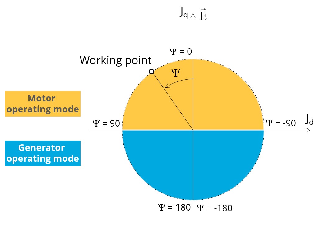
This input is available only if the generator operating mode is selected. Considering the vector diagram shown below, the “Control angle” is the angle between the electromotive force (E) and the electrical current (J) (Ψ = angle (E, J)).

Figure 1. Definition of the control angle Ψ

In the backend of FluxMotor, the control angle is varied within a research zone to find the value allows achieving the desired working point P-Pf-U-N. This research zone is discretized linearly based on the “Number of computations for control angle.”

The machine's performance is represented by the response surfaces of field current and control angle. An optimization algorithm uses these response surfaces to determine the field current and control angle that provide the required P-Pf-U-N performance. Thus, the “Number of computations for control angle” is crucial for the optimizer's accuracy.

Note: For the best compromise between computing time and accuracy, set the “Number of computations for control angle” to 13.

If higher accuracy is needed, increase this value accordingly, keeping in mind that higher values will require more computing time.

No. comp. / ripple period

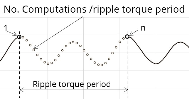
The number of computations per ripple torque period is considered to perform a “Ripple torque analysis”.

The user input “No. comp. / ripple period” (Number of computations per ripple torque period) influences the accuracy of results (computation of the peak-peak ripple torque) and the computation time.

The default value is equal to 30. The minimum allowed value is 25. The default value provides a good compromise between the accuracy of results and computation time.

Figure 2. Definition of the number of computations per ripple torque period

Skew model – No. of layers

When the rotor magnets or the stator slots are skewed, the number of layers used in Altair Flux Skew environment to model the machine can be modified: “Skew model - No. of layers” (Number of layers for modelling the skewing in Flux Skew environment).

Note: When there is magnet step skew topology, the number of layers is defined at the design level.

Rotor initial position

By default, the “Rotor initial position” is set to “Auto”.

When the “Rotor initial position mode” is set to “Auto”, the initial position of the rotor is automatically defined by an internal process.

The resulting relative angular position corresponds to the alignment between the axis of the stator phase 1 (reference phase) and the direct axis of the rotor.

When the “Rotor initial position” is set to “User input” (i.e. toggle button on the right), the initial position of the rotor considered for computation must be set by the user in the field « Rotor initial position ». The default value is equal to 0. The range of possible values is [-360, 360].

Notice: The computations are performed by considering the relative angular position between the rotor and stator.

This relative angular position corresponds to the angular distance between the direct axis of the rotor north pole and the axis of the stator phase 1 (reference phase).

The value of the rotor D-axis location, which is automatically defined for each saliency part.

Below is illustrated the Rotor and stator phase relative position

The relative angular position between the axis of the stator phase 1 (reference phase) and the rotor D-axis position must be controlled to perform the tests. See the picture below which will allow defining the working point of the machine.

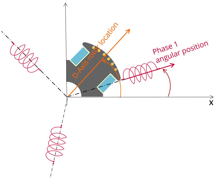
Figure 3. Definition of rotor initial position – Rules for direction

The winding axis of the reference phase is defined from the phase shift of the first electrical harmonic of the magneto motive force (M.M.F.).

Mesh order

To get the results, Finite Element Modelling computations are performed.

The geometry of the machine is meshed.

Two levels of meshing can be considered: First order and second order.

This parameter influences the accuracy of results and the computation time.

By default, second order mesh is used.

Airgap mesh coefficient

The advanced user input “Airgap mesh coefficient” is a coefficient which adjusts the size of mesh elements inside the airgap. When the value of “Airgap mesh coefficient” decreases, the mesh elements get smaller, leading to a higher mesh density inside the airgap, increasing the computation accuracy.

The imposed Mesh Point (size of mesh elements touching points of the geometry), inside the Altair Flux software, is described as:

MeshPoint = (airgap) x (airgap mesh coefficient)

Airgap mesh coefficient is set to 1.5 by default.

The variation range of values for this parameter is [0.05; 2].

0.05 giving a very high mesh density and 2 giving a very coarse mesh density.

CAUTION: Be aware, a very high mesh density does not always mean a better result quality. However, this always leads to a huge number of nodes in the corresponding finite element model. So, it means a need for huge numerical memory and increases the computation time considerably.

The impact of the airgap mesh coefficient on resultant meshing is illustrated bellow: