Inputs
Standard inputs ––––--
Operating quadrants
It defines the quadrants in the Jd - Jq plane, where the test will be carried out. By default, the only considered quadrant is the 2nd one (i.e., the grid is only defined for negative values of the current in the d axis and positive ones in the q axis). This corresponds to the motor behavior of the machine.
Options allow computing and displaying 1, 2 or 4 quadrants.
Among the standard inputs, the operating quadrants can be selected.
This allows defining the quadrants in the Jd-Jq plane, where the test will be carried out.
By default, the only considered quadrant is the 2nd one (i.e., the grid is only defined for negative values of the current in the d axis and positive ones in the q axis). This corresponds to the motor behavior of the machine.
The other possible values for this input are: “2nd and 3rd “, “1st and 2nd “and “all”.
Current definition mode
There are 2 common ways to define the electrical current.
Electrical current can be defined by the current density in electric conductors.
In this case, the current definition mode should be « Density ».
Electrical current can be defined directly by indicating the value of the line current (the RMS value is required).
In this case, the current definition mode should be « Current ».
Max. line current, h1 rms
Max. current dens. h1, rms
Maximum speed
The analysis of test results is performed over a given speed range, to evaluate losses as a function of speed like iron losses, mechanical losses, and total losses.
The speed range is fixed between 0 and the maximum speed to be considered « Maximum speed » (Maximum speed).
Rotor position dependency
Advanced inputs ––––--
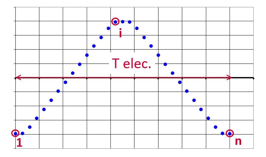
No. computed elec. periods
The user input “No. computed elec. periods” (Number of computed electrical periods) only required with rotor position dependency set to “Yes”) influences the computation time of the results.
The default value is equal to 0.5. The maximum allowed value is 1 according to the fact that computation is done to characterize steady state behavior based on magnetostatic finite element computation. The default value provides a good compromise between the accuracy of results and computation time.
No. comp. / elec. period
In general, the user input “No. comp. / elec. period” (Number of computed electrical periods) only required with rotor position dependency set to “Yes” influences the accuracy of results (computation of the peak-peak ripple torque, iron losses…) and the computation time.
No. comp. for Jd,Jq
To get maps in the Jd-Jq plan, a grid is defined. The number of computation points along the d-axis and q-axis can be defined with the user input « No. comp. for current Jd, Jq » (Number of computations per quadrant for D-axis and Q-axis phase currents).
The default value is equal to 5. This default value provides a good compromise between the accuracy of results and computation time. The minimum allowed value is 5.
No. comp. for speed
The number of computations for speed corresponds to the number of points to consider in the range of speed. It can be defined via the user input “No. comp. for speed” (Number of computations for speed).
The default value is equal to 10. The minimum allowed value is 5.
Skew model – No. of layers
Mesh order
To get the results, Finite Element Modelling computations are performed.
The geometry of the machine is meshed.
Two levels of meshing can be considered: First order and second order.
This parameter influences the accuracy of results and the computation time.
By default, second order mesh is used.
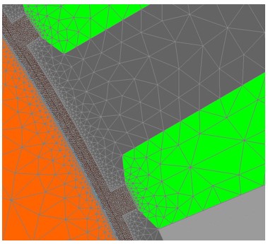
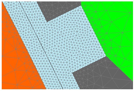
Airgap mesh coefficient
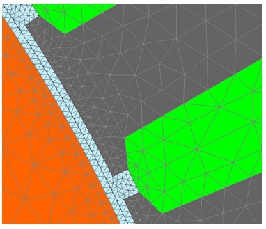
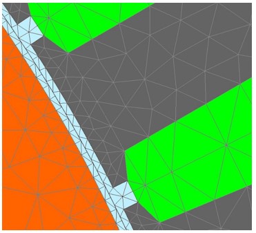
The advanced user input “Airgap mesh coefficient” is a coefficient which adjusts the size of mesh elements inside the airgap. When the value of “Airgap mesh coefficient” decreases, the mesh elements get smaller, leading to a higher mesh density inside the airgap, increasing the computation accuracy.
The imposed Mesh Point (size of mesh elements touching points of the geometry), inside the Altair Flux software, is described as:
MeshPoint = (airgap) x (airgap mesh coefficient)
Airgap mesh coefficient is set to 1.5 by default.
The variation range of values for this parameter is [0.05; 2].
The impact of the airgap mesh coefficient on resultant meshing is illustrated bellow:
Rotor initial position mode
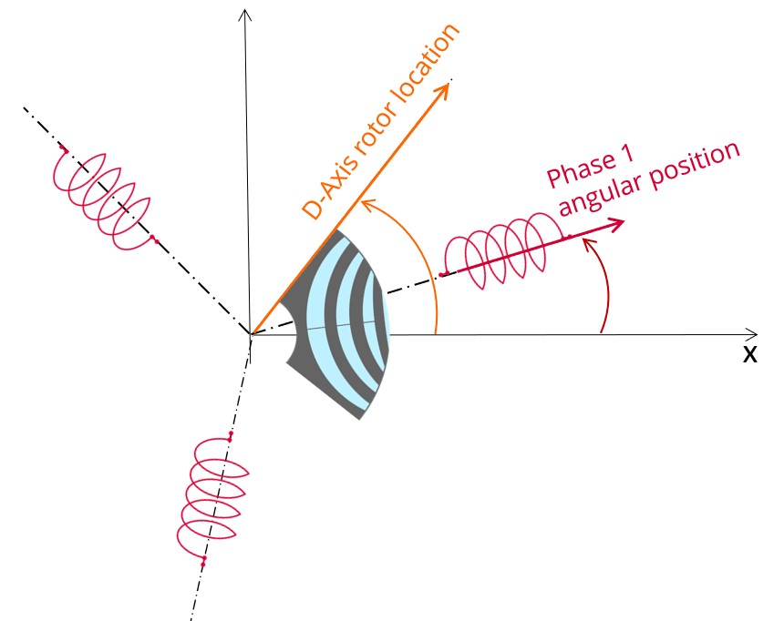
The computations are performed by considering a relative angular position between rotor and stator.
This relative angular position corresponds to the angular distance between the direct axis of the rotor north pole and the axis of the stator phase 1 (reference phase).
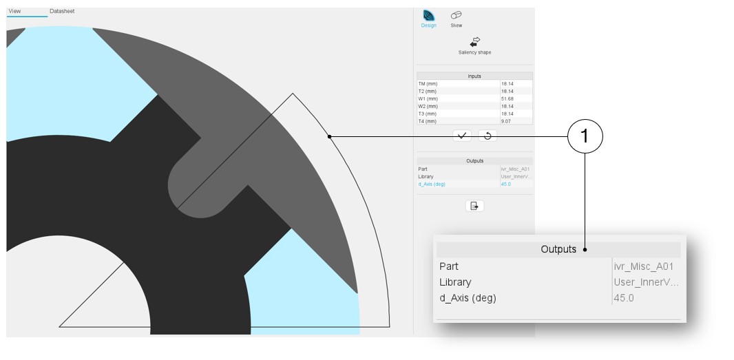
The value of the rotor d-axis location, which is automatically defined, for each saliency part, in Part Factory, can be visualized in the output parameters in the saliency area of Motor Factory – Design environment.
Rotor initial position
The winding axis of the reference phase is defined from the phase shift of the first electrical harmonic of the magneto motive force (M.M.F.).
The rotor d-axis location is characterized by the saliency topology.
The relative angular position between the axis of the stator phase 1 (reference phase) and the rotor D-axis position must be controlled to perform the tests. See the picture below which will allow defining the working point of the machine.
Here is the representation below of the rotor and stator phase relative position.
The relative angular position between the axis of the stator phase 1 (reference phase) and the rotor D-axis position must be controlled to perform the tests.
The winding axis of the reference phase is defined from the phase shift of the first electrical harmonic of the magneto motive force (M.M.F.).
This allows us to define the working point of the machine.
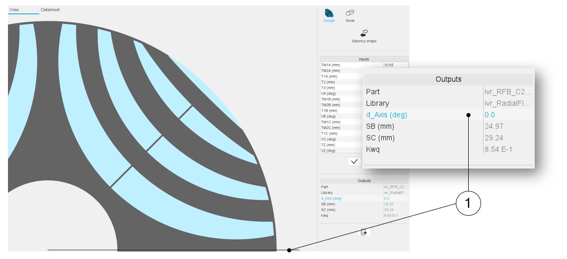
The rotor d-axis location is an output parameter (read only data) of saliency parts. It completes the description of the topology, and it is automatically used to define the relative position between the axis of the stator phase 1 (reference phase) and the rotor D-axis position for performing the tests when needed.