Inputs

Standard inputs ––––--

Speed

Operating speed of the machine is the only standard input parameter to be used in the back-EMF test.

Note: Once the computation is performed, it is possible to change the speed and update the results instantaneously.

Advanced inputs ––––--

No. comp. / elec. period

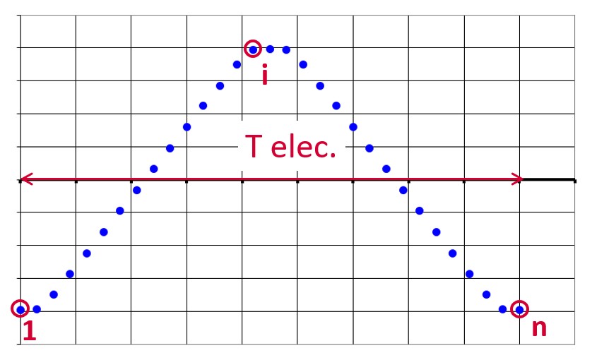
In general, the user input “No. comp. / elec. period” (Number of computed electrical periods) only required with rotor position dependency set to “Yes” influences the accuracy of results (computation of the peak-peak ripple torque, iron losses…) and the computation time.

The default value is equal to 40. The minimum recommended value is 20. The default value provides a good balance between the accuracy of results and the computation time.

Note: The real number of computations per electrical period can be equal to the requested one +/- 1. That is due to our internal computation process since the raw computation is performed over one electrical half period. The result on a whole electrical period is rebuilt from the raw data.

Figure 1. Number of computations per electrical period

Max. harmonic order

To get the Back-EMF versus time, the flux through each phase of the machine is computed versus rotor angular position.

Harmonics are extracted from the frequency analysis (F.F.T. Fast Fourier Transform) of the Back-EMF signal versus time.

The order of harmonics displayed on bar graphs and in tables can be selected with this advanced user input parameter “Max. harmonic order” (Maximum harmonic order selected for visualization).

Note: From mathematical point of view, the maximum allowed harmonic order depends on the number of computations per electrical period. In case of a too small number of computations per electrical period, the maximum harmonic order considered will be lower than the one set up by the user.

The default value is equal to 20. The minimum allowed value is 1.

Rotor initial position

By default, the “Rotor initial position” is set to “Auto”

(except in the test Characterization / Cogging where it is a user input whose default value is 0).

When the “Rotor initial position mode” is set to “Auto”, the initial position of the rotor is automatically defined by an internal process of FluxMotor.

The resulting relative angular position corresponds to the alignment between the axis of the stator phase 1 (reference phase) and the direct axis of the rotor north pole.

When the “Rotor initial position” is set to “User input” (i.e. toggle button on the right), the initial position of the rotor considered for computation must be set by the user in the field « Rotor initial position ». The default value is equal to 0. The range of possible values is [-360, 360].

Notice: The relative angular position between the axis of the stator phase 1 (reference phase) and the direct axis of the rotor north pole must be controlled to perform the tests. See the picture below. That allows defining the working point of the machine.

Figure 2. Definition of rotor initial position – Rules for direction

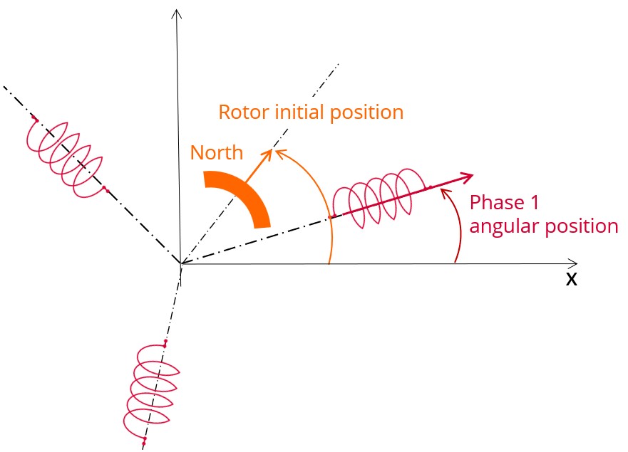
The winding axis of the reference phase is defined from the phase shift of the first electrical harmonic of the magneto motive force (M.M.F.).

By convention, a field pole "North” corresponds to a magnetic flux density vector oriented towards exterior of the rotor.

Note: In the test Characterization / Cogging there is a user input whose default value is 0, no Auto mode available.

Skew model – No. of layers

When the rotor magnets or the stator slots are skewed, the number of layers used in Altair Flux Skew environment to model the machine can be modified: “Skew model - No. of layers” (Number of layers for modelling the skewing in Flux Skew environment).

Note: When there is magnet step skew topology, the number of layers is defined at the design level.

Mesh order

To get the results, Finite Element Modelling computations are performed.

The geometry of the machine is meshed.

Two levels of meshing can be considered: First order and second order.

This parameter influences the accuracy of results and the computation time.

By default, second order mesh is used.

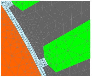
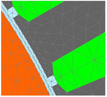
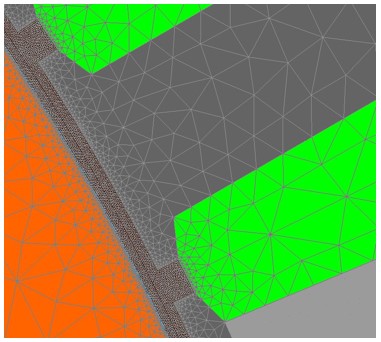
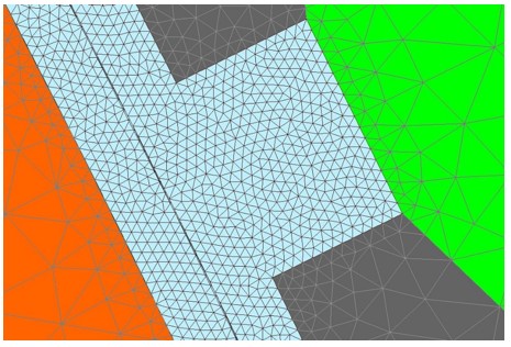
Airgap mesh coefficient

The advanced user input “Airgap mesh coefficient” is a coefficient which adjusts the size of mesh elements inside the airgap. When the value of “Airgap mesh coefficient” decreases, the mesh elements get smaller, leading to a higher mesh density inside the airgap, increasing the computation accuracy.

The imposed Mesh Point (size of mesh elements touching points of the geometry), inside the Altair Flux software, is described as:

MeshPoint = (airgap) x (airgap mesh coefficient)

Airgap mesh coefficient is set to 1.5 by default.

The variation range of values for this parameter is [0.05; 2].

0.05 giving a very high mesh density and 2 giving a very coarse mesh density.

CAUTION: Be aware, a very high mesh density does not always mean a better result quality. However, this always leads to a huge number of nodes in the corresponding finite element model. So, it means a need for huge numerical memory and increases the computation time considerably.

The impact of the airgap mesh coefficient on resultant meshing is illustrated bellow:

Figure 3. Airgap mesh coefficient = 0.45 = default value

Figure 6. Airgap mesh coefficient = 0.1 (zoomed view)