Common area

Rotor initial position

By default, the “Rotor initial position” is set to “Auto”

(except in the test Characterization / Cogging where it is a user input whose default value is 0).

When the “Rotor initial position mode” is set to “Auto”, the initial position of the rotor is automatically defined by an internal process of FluxMotor.

The resulting relative angular position corresponds to the alignment between the axis of the stator phase 1 (reference phase) and the direct axis of the rotor north pole.

When the “Rotor initial position” is set to “User input” (i.e. toggle button on the right), the initial position of the rotor considered for computation must be set by the user in the field « Rotor initial position ». The default value is equal to 0. The range of possible values is [-360, 360].

Notice: The relative angular position between the axis of the stator phase 1 (reference phase) and the direct axis of the rotor north pole must be controlled to perform the tests. See the picture below. That allows defining the working point of the machine.

Figure 1. Definition of rotor initial position – Rules for direction

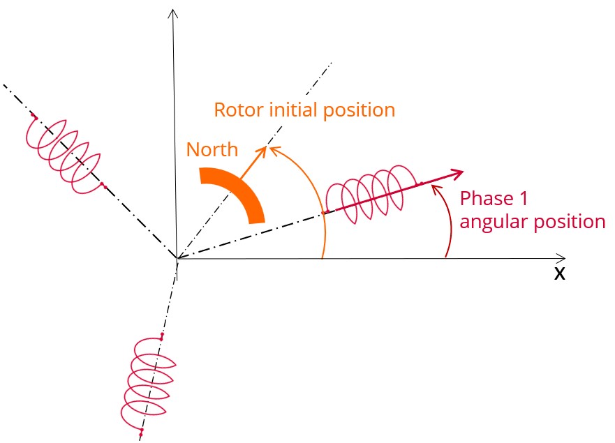
The winding axis of the reference phase is defined from the phase shift of the first electrical harmonic of the magneto motive force (M.M.F.).

By convention, a field pole "North” corresponds to a magnetic flux density vector oriented towards exterior of the rotor.

Note: In the test Characterization / Cogging there is a user input whose default value is 0, no Auto mode available.

Mesh order

To get the results, Finite Element Modelling computations are performed.

The geometry of the machine is meshed.

Two levels of meshing can be considered: First order and second order.

This parameter influences the accuracy of results and the computation time.

By default, second order mesh is used.

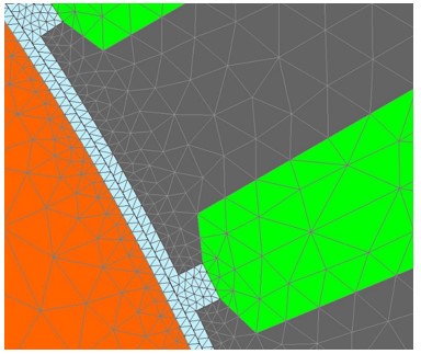
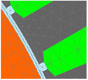
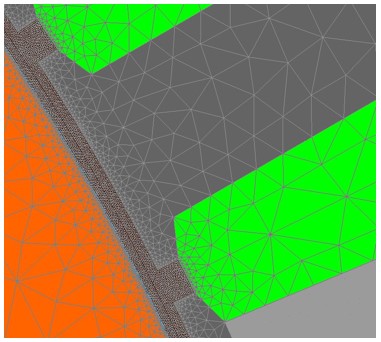
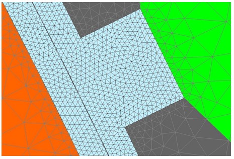
Airgap mesh coefficient

The advanced user input “Airgap mesh coefficient” is a coefficient which adjusts the size of mesh elements inside the airgap. When the value of “Airgap mesh coefficient” decreases, the mesh elements get smaller, leading to a higher mesh density inside the airgap, increasing the computation accuracy.

The imposed Mesh Point (size of mesh elements touching points of the geometry), inside the Altair Flux software, is described as:

MeshPoint = (airgap) x (airgap mesh coefficient)

Airgap mesh coefficient is set to 1.5 by default.

The variation range of values for this parameter is [0.05; 2].

0.05 giving a very high mesh density and 2 giving a very coarse mesh density.

CAUTION: Be aware, a very high mesh density does not always mean a better result quality. However, this always leads to a huge number of nodes in the corresponding finite element model. So, it means a need for huge numerical memory and increases the computation time considerably.

The impact of the airgap mesh coefficient on resultant meshing is illustrated bellow:

Figure 2. Airgap mesh coefficient = 0.45 = default value

Figure 5. Airgap mesh coefficient = 0.1 (zoomed view)

Skew model – No. of layers

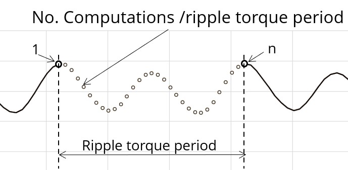
When the rotor magnets or the stator slots are skewed, the number of layers used in Altair Flux Skew environment to model the machine can be modified: “Skew model - No. of layers” (Number of layers for modelling the skewing in Flux Skew environment).

Note: When there is magnet step skew topology, the number of layers is defined at the design level.

No. comp. / ripple period

The number of computations per ripple torque period is considered to perform a “Ripple torque analysis”.

The user input “No. comp. / ripple period” (Number of computations per ripple torque period) influences the accuracy of results (computation of the peak-peak ripple torque) and the computation time.

The default value is equal to 30. The minimum allowed value is 25. The default value provides a good compromise between the accuracy of results and computation time.

Figure 6. Definition of the number of computations per ripple torque period

No. comp. / elec. period

In general, the user input “No. comp. / elec. period” (Number of computed electrical periods) only required with rotor position dependency set to “Yes” influences the accuracy of results (computation of the peak-peak ripple torque, iron losses…) and the computation time.

The default value is equal to 40. The minimum recommended value is 20. The default value provides a good balance between the accuracy of results and the computation time.

Note: The real number of computations per electrical period can be equal to the requested one +/- 1. That is due to our internal computation process since the raw computation is performed over one electrical half period. The result on a whole electrical period is rebuilt from the raw data.

Figure 7. Number of computations per electrical period

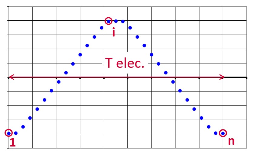
No. computed elec. periods

The user input “No. computed elec. periods” (Number of computed electrical periods) only required with rotor position dependency set to “Yes”) influences the computation time of the results.

The default value is equal to 0.5. The maximum allowed value is 1 according to the fact that computation is done to characterize steady state behavior based on magnetostatic finite element computation. The default value provides a good compromise between the accuracy of results and computation time.

Current definition mode

There are 2 common ways to define the electrical current.

Electrical current can be defined by the current density in electric conductors.

In this case, the current definition mode should be « Density ».

Electrical current can be defined directly by indicating the value of the line current (the RMS value is required).

In this case, the current definition mode should be « Current ».

Line current h1, rms

When the choice of current definition mode is “Current”, the rms value of the line current supplied to the machine: “Line current, h1 rms” (Line current, first harmonic rms value) must be provided.

Max. line current, h1 rms

When the choice of current definition mode is “Current”, the maximum rms value of the line current supplied to the machine “Max. line current, h1 rms” (Maximum line current, first harmonic rms value) must be provided.

Note: The number of parallel paths and the winding connections are automatically considered in the results.

Current density h1, rms

When the choice of current definition mode is “Density”, the rms value of the current density in electric conductors “Current density, h1 rms” (Current density in conductors, first harmonic rms value) must be provided.

Note: The number of parallel paths and the winding connection are automatically considered in the results.

Max. current dens. h1, rms

When the choice of current definition mode is “Density”, the maximum rms value of the current density in electric conductors “Max. current dens., h1 rms” (Maximum current density in conductors, first harmonic rms value) must be provided.

Note: The number of parallel paths and the winding connection are automatically considered in the results.

Max. Line-Line voltage, h1 rms

To supply the machine the rms value of the maximum Line-Line voltage: “Max. Line-Line voltage, h1 rms” (Maximum Line-Line voltage, first harmonic rms value) must be provided.

Note: The number of parallel paths and the winding connection are automatically considered in the results.

No. comp. for Jd,Jq

To get maps in the Jd-Jq plan, a grid is defined. The number of computation points along the d-axis and q-axis can be defined with the user input « No. comp. for current Jd, Jq » (Number of computations per quadrant for D-axis and Q-axis phase currents).

The default value is equal to 5. This default value provides a good compromise between the accuracy of results and computation time. The minimum allowed value is 5.

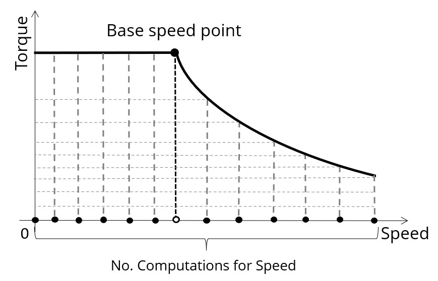
No. comp. for speed

The “No. comp. for speed” (Number of computations for speed) corresponds to the number of points to be considered in the speed range from 0 to the maximum speed.

Half of these points are distributed from 0 to the base speed. The remaining points are distributed from the base speed to the maximum speed.

In both cases, base speed is considered as an additional point.

Note: If the user input parameter “No. comp. for speed” is an odd number, one discretization point is automatically removed.

Figure 8. Definition of the number of computations for speed

The default value is equal to 15, the minimum allowed value is 5. The maximum recommended value is 40.

Note: Increasing the number of computations can improve the convergence of the optimization used to define the torque-speed curve and the efficiency map. However, that also means longer computation time.

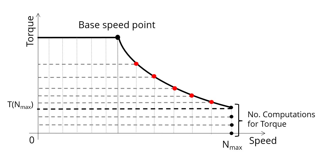
No. comp. for torque

For the speed range [Nbase; Nmax.], the number of computations for torque is imposed by the number of computations for speed in the speed range [Nbase; Nmax.] (Red points in the image shown below).

The advanced user input parameter “No. comp. for torque” allows to finalize the grid within the torque range [0, T (Nmax.)] at the maximum speed (Black points in the image shown below).

The default value is equal to 7. The minimum allowed value is 3. The maximum recommended value is 20.

Figure 9. Definition of the number of computations for torque – MTPV command mode

Max. engine order

Two kinds of inputs are possible: either set an engine order or a number of points per electrical period. Define the Max. engine order (Maximum engine order) or the No. points / elec. period (Number of points per electric period).

When decomposing the Maxwell pressure, applied on the stator, to get its harmonic contributions, the “max. engine order” (Maximum engine order) is required to compute its decomposition in function of the time.

At a practical point of view, when the maximum engine order is equal to N, that leads to consider 2*N computation points over a complete rotation period of the rotor.

Note: The input "Engine order" is in connection with the frequency of vibration.

"Engine order" refers to a mechanical revolution period of the motor whereas frequency refers to the considered electrical period.

Obviously, both are linked with speed.

For instance, radiated sound power can be displayed either by considering frequency or engine order.

No. points / elec. period

The second possibility is to set a “No. points / elec. Period” meaning a number of points per electrical period.

For transient computations the minimum needed number of points per electrical period is 40.

So, when the engine order is not high enough to reach this constraint, It is automatically modified to get 40 computation points per electrical period.

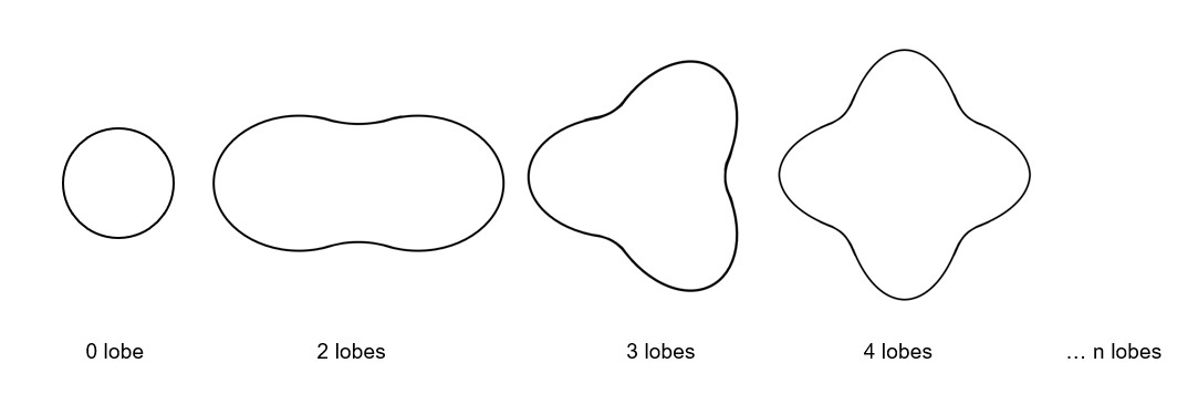
Max. mode / spatial order

The “max. mode / spatial order” (Maximum mode / spatial order) input allows the user to define the number of modes to be considered for the acoustic structural analysis. If the user selects 25, it means that the highest number of lobes in the stator deformation will be equal to 25 lobes. All deformations corresponding to more than 25 lobes will be dismissed.

Figure 10. Number of lobes of the stator mechanical structure

No. points / tooth pitch

The “No. comp. / tooth pitch” (Number of computations per tooth pitch) allows to choose the number of Maxwell pressure evaluations per tooth. The more points selected, the more accurate the Maxwell pressure harmonic decomposition will be.

Advice for use

The modal analysis as well as the radiation efficiency are based on an analytical computation where the stator of the machine is considered as a vibrating cylinder.

The considered cylinder behavior is weighted by the additional masses like the fins or the winding and the subtractive masses like the slots and the cooling circuit holes.

This assumption allows to get fast evaluation of the behavior of machine in connection to NVH. In no way this can replace a mechanical Finite Element modeling and simulation.

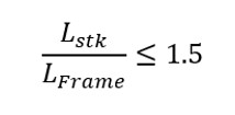
Among possible reasons for deviations of results can be the following ones:

The limits of the analytical model are reached or overpassed
Unusual topology and/or dimensions of the teeth/slots
Complexity of the stator-frame structure when it is composed with several components for instance
The ratio between the total length of the frame Lframe and the stack length of the machine Lstk in any case, this ratio must be lower than 1.5: