Inputs
Standard inputs ––––--
Operational inductance order
The operational inductance order (Operational inductance order) can be either “1st” order or “2nd” order.
This choice depends on the squirrel cage topology but also on the results obtained with the 1st order model. When the first order model doesn’t allow getting good fitting between computation results from Finite Elements computations of the operational inductance and those got with the resulting analytical model, the 2nd order is needed.
By default, this input is set to “1st order”.
Model evaluation
The “Model evaluation” of the resulting equivalent scheme (Model evaluation of SSFR model by a direct starting test) is possible by performing a direct starting of the motor.
The starting is operated with a start winding connection.
When the “Model evaluation” is “Yes”, quantities like speed, electromagnetic torque and stator current are computed, and displayed based on the calculated model.
By default, this input is set to “No”.
Op. Line-Line voltage, h1 rms
The rms value of the Line-Line voltage supplying the machine: “Op. Line-Line voltage, h1 rms” (Line-Line voltage, first harmonic rms value) must be provided to compute the starting of the motor.
- The number of parallel paths is automatically considered in the results.
- The starting is always operated by considering a start winding connection.
Op. power supply freq.
The value of the power supply frequency of the machine: “Op. power supply freq.” (Operating power supply frequency to evaluate the SSFR model) must be provided.
The power supply frequency is the electrical frequency applied at the terminals of the machine.
Add. moment of inertia
An additional moment of inertia: “Add. moment of inertia” (Additional moment of inertia) can be added for considering an additional moment of inertia of a load on the shaft line for instance.
By default, this input is equal to 0 N.m.
Max. evaluation duration
The Max. evaluation duration (Maximum evaluation duration) allows us to limit the computation time needed to evaluate the starting of the motor.
However, an internal process detects automatically when the motor reaches the steady state after the transient starting phase.
When the time required for reaching the steady state is lower than the maximum evaluation duration, the computation ends automatically. When the steady state is established instead of computing the maximum evaluation duration it ends automatically.
By default, this input is equal to 1 second.
Advanced inputs ––––--
Linear permeability distribution
Two methods allow defining the permeability in the magnetic circuit of the machine; either the magnetic permeability is constant in the stator, rotor and shaft or the magnetic permeability is linked to the magnetic state of the machine when running at a working point.
When the “Linear permeability distribution” mode is “Constant”, the relative magnetic permeability must be defined for the stator, the rotor, and the shaft.
When the “Linear permeability distribution” mode is “Working point” the characteristics of the working point must be defined with the Line-Line voltage U, the power supply frequency f and the speed N.
Then, the magnetic permeability mapping of a motor is done at the selected working point (U, f, N).
The resulting map of permeability is then applied to the model while performing the frequency analysis. This is what we call the frozen permeability method.
Stator permeability
This input allows to set the value of the magnetic permeabilities for the stator. To meet the requirements of the test assumptions, the computations with Finite Elements are operated by considering linear ferromagnetic materials.
The relative permeability of the stator “Stator permeability” (stator magnetic relative permeability) is by default set to Auto. In this auto mode, the applied stator relative permeability is computed by an internal process (see illustration in below section) in case of a nonlinear magnetic material since the SSFR test is based on the principle that magnetic materials need to be linear.
In case of a linear magnetic material, the stator permeability is the one defined in the material properties (no internal computation is necessary).
The user can enter his own stator permeability by using the toggle button added for this purpose.
This value allows to perform the SSFR test.
Rotor permeability
This input allows to set the value of the magnetic permeabilities for the rotor. To meet the requirements of the test assumptions, the computations with Finite Elements are operated by considering linear ferromagnetic materials
The relative permeability of the rotor “Rotor permeability” (rotor magnetic relative permeability) is defined as the stator permeability by two modes. An auto mode and a user mode. By default, it is set to Auto.
This value allows to perform the SSFR test.
Shaft permeability
This input allows us to set the value of the magnetic permeabilities for the shaft. To meet the requirements of the test assumptions, the computations with Finite Elements are operated by considering linear ferromagnetic materials.
Materials magnetic properties
To meet the requirements of the test assumptions, the computations with Finite Elements are operated by considering linear ferromagnetic materials.
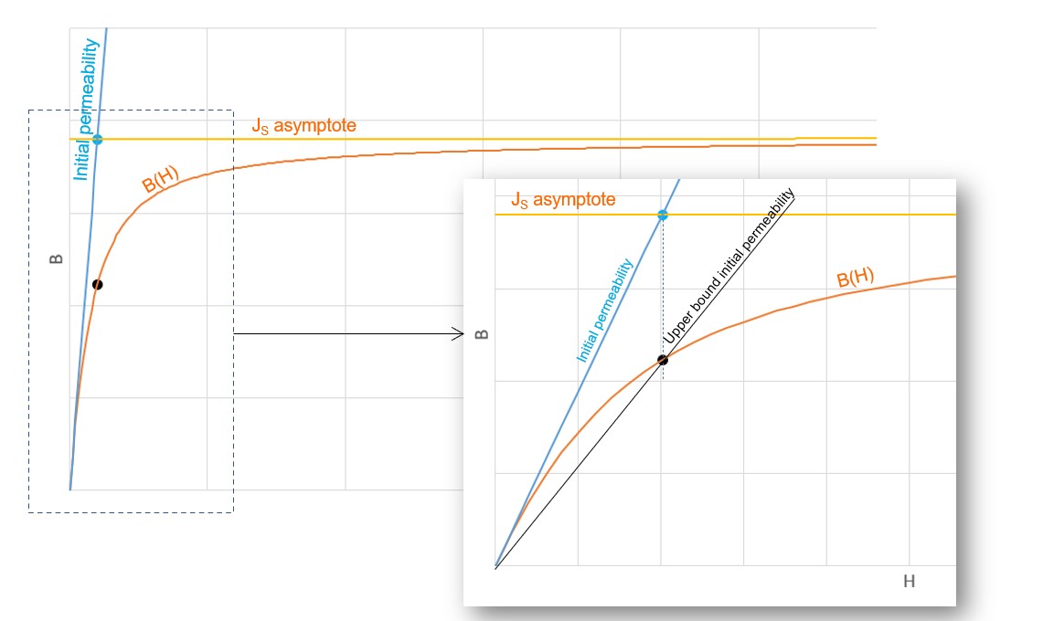
The constant value of each material magnetic permeability is computed by considering a mean value in the very first part of the considered B(H) curve.
At a practical point of view, the constant magnetic permeability used in the computation is the average value of initial and the upper bound permeability defined as below illustrated.
WP – Line-Line voltage, h1 rms
When the “Linear permeability distribution” mode is “working point, it means that the frequency analysis to compute the operational inductance - L(p) – is based on a working point defined with the Line-Line voltage U, the power supply frequency f, and the speed N.
The working point – Line-Line voltage, first harmonic rms value (WP – Line-Line voltage, h1 rms) must be provided.
WP – power supply frequency
When the “Linear permeability distribution” mode is “working point, it means that the frequency analysis to compute the operational inductance - L(p) – is based on a working point defined with the Line-Line voltage U, the power supply frequency f, and the speed N.
The working point – power supply frequency (WP – power supply frequency) must be provided.
WP – Slip
When the “Linear permeability distribution” mode is “working point, it means that the frequency analysis to compute the operational inductance - L(p) – is based on a working point defined with the Line-Line voltage U, the power supply frequency f, and the speed N.
The working point – slip (WP – Slip) must be provided.
No. comp. / elec. period
To get the quantities like the speed, torque and current versus time, an analytical computation is performed.
The number of computations per electrical period “No. comp. / elec. period” (Number of computations per electrical period) influences the accuracy of results and the computation time.
The default value is equal to 50. The minimum allowed value is 40. This default value provides a good compromise between the accuracy of results and computation time.
SSFR voltage, h1 rms
- The number of parallel paths is automatically considered in the results.
- The test is always operated by considering a star winding connection.
By default, this input is equal to 0.2 volt.
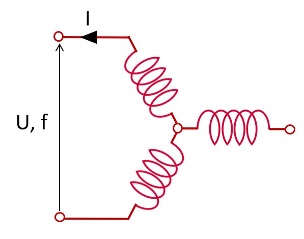
The test procedure for performing the SSFR test consists in applying a fixed low voltage source between two terminals of the machine armature winding (Star winding connection) over a range of frequencies. SSFR voltage corresponds to the voltage source magnitude (U) applied.
For additional information please refer to the main principles of computation, section.
Skew model – No. of layers
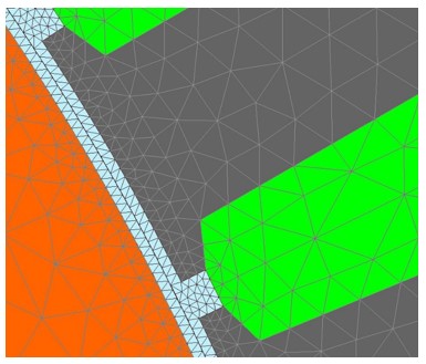
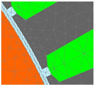
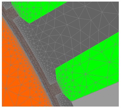
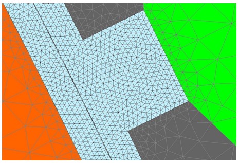
Airgap mesh coefficient
The advanced user input “Airgap mesh coefficient” is a coefficient which adjusts the size of mesh elements inside the airgap. When the value of “Airgap mesh coefficient” decreases, the mesh elements get smaller, leading to a higher mesh density inside the airgap, increasing the computation accuracy.
The imposed Mesh Point (size of mesh elements touching points of the geometry), inside the Altair Flux software, is described as:
MeshPoint = (airgap) x (airgap mesh coefficient)
Airgap mesh coefficient is set to 1.5 by default.
The variation range of values for this parameter is [0.05; 2].
The impact of the airgap mesh coefficient on resultant meshing is illustrated bellow: