Common area

Current definition mode

There are 2 common ways to define the electrical current.

Electrical current can be defined by the current density in electric conductors.

In this case, the current definition mode should be « Density ».

Electrical current can be defined directly by indicating the value of the line current (the RMS value is required).

In this case, the current definition mode should be « Current ».

Line current, h1 rms

The rms value of the Line current supplying the machine: “Line current, h1 rms” (Line current, harmonic rms value) must be provided.

Note: The number of parallel paths and the winding connections are automatically considered in the results.

Line-Line voltage, h1 rms

The rms value of the Line-Line voltage supplying the machine: “Line-Line voltage, h1 rms” (Line-Line voltage, first harmonic rms value) must be provided.

Note: The number of parallel paths and the winding connection are automatically considered in the results.

Power supply frequency

The value of the power supply frequency of the machine: “Power supply frequency” (Power supply frequency) must be provided.

The power supply frequency is the electrical frequency applied at the terminals of the machine.

Airgap mesh coefficient

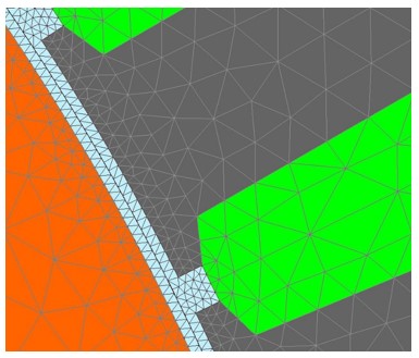
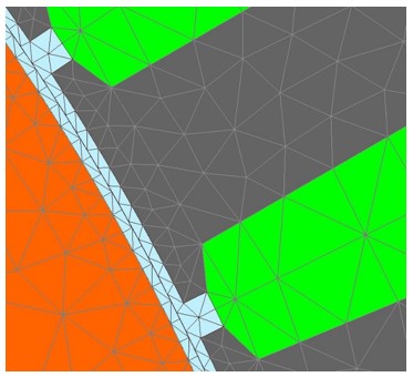
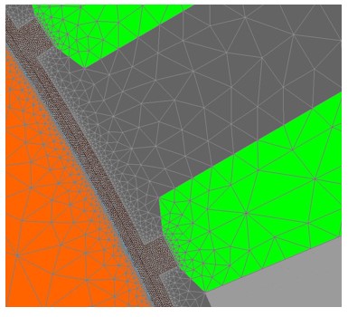
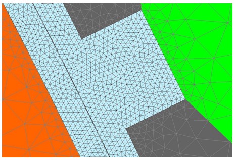
The advanced user input “Airgap mesh coefficient” is a coefficient which adjusts the size of mesh elements inside the airgap. When the value of “Airgap mesh coefficient” decreases, the mesh elements get smaller, leading to a higher mesh density inside the airgap, increasing the computation accuracy.

The imposed Mesh Point (size of mesh elements touching points of the geometry), inside the Altair Flux software, is described as:

MeshPoint = (airgap) x (airgap mesh coefficient)

Airgap mesh coefficient is set to 1.5 by default.

The variation range of values for this parameter is [0.05; 2].

0.05 giving a very high mesh density and 2 giving a very coarse mesh density.

CAUTION: Be aware, a very high mesh density does not always mean a better result quality. However, this always leads to a huge number of nodes in the corresponding finite element model. So, it means a need for huge numerical memory and increases the computation time considerably.

The impact of the airgap mesh coefficient on resultant meshing is illustrated bellow:

Figure 1. Airgap mesh coefficient = 0.45 = default value

Figure 4. Airgap mesh coefficient = 0.1 (zoomed view)

Mesh order

To get the results, Finite Element Modelling computations are performed.

The geometry of the machine is meshed.

Two levels of meshing can be considered: First order and second order.

This parameter influences the accuracy of results and the computation time.

By default, second order mesh is used.

Skew model – No. of layers

When the rotor magnets or the stator slots are skewed, the number of layers used in Altair Flux Skew environment to model the machine can be modified: “Skew model - No. of layers” (Number of layers for modelling the skewing in Flux Skew environment).

Note: When there is magnet step skew topology, the number of layers is defined at the design level.

EM – No. comp. for speed

The “EM - No. comp. for speed” (Efficiency map - Number of computations for speed) corresponds to the number of points to be considered in the speed range from 0 to the maximum speed.

Half of these points are distributed from 0 to the base speed. The remaining points are distributed from the base speed to the maximum speed.

In both cases, base speed is considered as an additional point.

Note: If the user input parameter “No. comp. for speed” is an odd number, one discretization point is automatically removed.

Figure 5. Definition of the number of computations for speed

The default value is equal to 20. The minimum allowed value is 10 while the maximum recommended value is 40.

Note: Increasing the number of computations can improve the convergence of the optimization used to define the torque-speed curve and the efficiency map. However, that also means longer computation time.

EM – No. comp. for torque

For the speed range [Nbase; Nmax.], the number of computations for torque is imposed by the number of computations for the defined speed range [Nbase; Nmax.] (Red points in the image shown below).

The advanced user input parameter “EM - No. comp. for torque” (Efficiency map - Number of computations for torque) allows to finalize the grid within the torque range [0, T (Nmax.)] at the maximum speed (Black points in the image shown below).

The default value is equal to 4. The minimum allowed value is 4 while the maximum recommended value is 10.

Figure 6. Definition of the number of computations for torque

No. comp. for speed

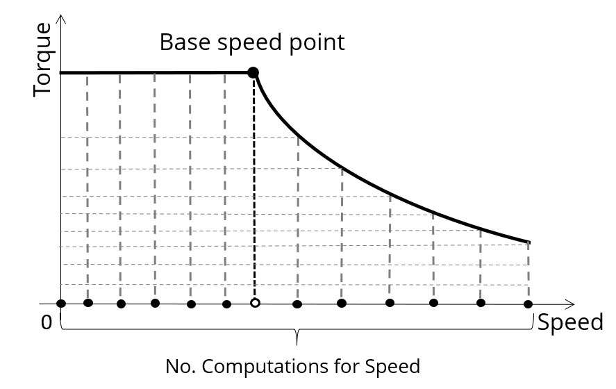
The “No. comp. for speed” (Number of computations for speed) corresponds to the number of points to be considered in the speed range from 0 to the maximum speed.

Half of these points are distributed from 0 to the base speed. The remaining points are distributed from the base speed to the maximum speed.

In both cases, base speed is considered as an additional point.

Note: If the user input parameter “No. comp. for speed” is an odd number, one discretization point is automatically removed.

Figure 7. Definition of the number of computations for speed

The default value is equal to 15, the minimum allowed value is 5. The maximum recommended value is 40.

Note: Increasing the number of computations can improve the convergence of the optimization used to define the torque-speed curve and the efficiency map. However, that also means longer computation time.

No. comp. for torque

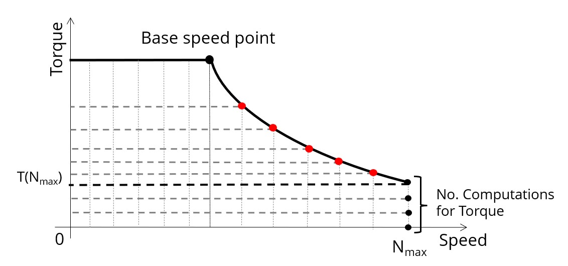
For the speed range [Nbase; Nmax.], the number of computations for torque is imposed by the number of computations for speed in the speed range [Nbase; Nmax.] (Red points in the image shown below).

The advanced user input parameter “No. comp. for torque” allows to finalize the grid within the torque range [0, T (Nmax.)] at the maximum speed (Black points in the image shown below).

The default value is equal to 7. The minimum allowed value is 3. The maximum recommended value is 20.

Figure 8. Definition of the number of computations for torque – MTPV command mode

Max. engine order

Two kinds of inputs are possible: either set an engine order or a number of points per electrical period. Define the Max. engine order (Maximum engine order) or the No. points / elec. period (Number of points per electric period).

When decomposing the Maxwell pressure, applied on the stator, to get its harmonic contributions, the “max. engine order” (Maximum engine order) is required to compute its decomposition in function of the time.

At a practical point of view, when the maximum engine order is equal to N, that leads to consider 2*N computation points over a complete rotation period of the rotor.

Note: The input "Engine order" is in connection with the frequency of vibration.

"Engine order" refers to a mechanical revolution period of the motor whereas frequency refers to the considered electrical period.

Obviously, both are linked with speed.

For instance, radiated sound power can be displayed either by considering frequency or engine order.

No. points / elec. period

The second possibility is to set a “No. points / elec. Period” meaning a number of points per electrical period.

For transient computations the minimum needed number of points per electrical period is 40.

So, when the engine order is not high enough to reach this constraint, It is automatically modified to get 40 computation points per electrical period.

Max. mode / spatial order

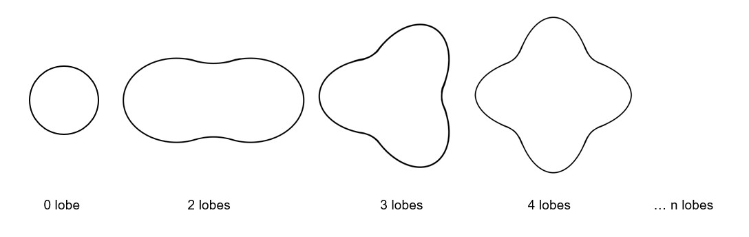
The “max. mode / spatial order” (Maximum mode / spatial order) input allows the user to define the number of modes to be considered for the acoustic structural analysis. If the user selects 25, it means that the highest number of lobes in the stator deformation will be equal to 25 lobes. All deformations corresponding to more than 25 lobes will be dismissed.

Figure 9. Number of lobes of the stator mechanical structure

No. points / tooth pitch

The “No. comp. / tooth pitch” (Number of computations per tooth pitch) allows to choose the number of Maxwell pressure evaluations per tooth. The more points selected, the more accurate the Maxwell pressure harmonic decomposition will be.

Displayed pressure range (dB)

The “displayed pressure range (dB)” (Displayed Maxwell pressure range) is only related to the displaying of results.

It allows to increase/decrease the range of non-zero contributions displayed in the Maxwell pressure harmonic decomposition map.

When one chooses a displayed pressure range equal to 50 dB, only the contributions within the range of 50 dB and below the maximum computed value is displayed.

Note: The absolute reference value Pref (expressed in Pa), which corresponds to 0 dB, is indicated in the working point table.

Considering this referent value Pref, one can compute any Maxwell pressure value PPa (expressed in Pa) from the ones expressed in Decibel PdB.

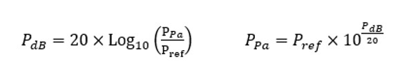
The relations between these quantities are illustrated below:

The default value is equal to 60. The range of possible values is [20;100].

Number of rotor turns

This input allows us to define the number of rotor revolutions to consider the slip as far as possible.

Higher is the number of rotor revolutions better will be the results. However, this value has a huge impact on the computation time.

The default value is equal to 5. This is a good compromise between computation time and quality of results.

The variation range of values for this parameter is [1; 10].

Advice for use

The modal analysis as well as the radiation efficiency are based on an analytical computation where the stator of the machine is considered as a vibrating cylinder.

The considered cylinder behavior is weighted by the additional masses like the fins or the winding and the subtractive masses like the slots and the cooling circuit holes.

This assumption allows to get fast evaluation of the behavior of machines in connection to NVH. In no way this can replace mechanical Finite Element modeling and simulation.

Among possible reasons for deviations of results can be the following ones:

The limits of the analytical model are reached or overpassed.
Unusual topology and/or dimensions of the teeth/slots
Complexity of the stator-frame structure when it is composed with several components for instance.
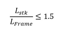
The ratio between the total length of the frame Lframe and the stack length of the machine Lstk in any case, this ratio must be lower than 1.5: