Package Modelica.​Blocks.​Examples
Library of examples to demonstrate the usage of package Blocks

Information

This package contains example models to demonstrate the usage of package blocks.

Extends from Modelica.​Icons.​ExamplesPackage (Icon for packages containing runnable examples).

Package Contents

Model Modelica.​Blocks.​Examples.​PID_Controller
Demonstrates the usage of a Continuous.LimPID controller

Information

This is a simple drive train controlled by a PID controller:

• The two blocks "kinematic_PTP" and "integrator" are used to generate the reference speed (= constant acceleration phase, constant speed phase, constant deceleration phase until inertia is at rest). To check whether the system starts in steady state, the reference speed is zero until time = 0.5 s and then follows the sketched trajectory.
• The block "PI" is an instance of "Blocks.Continuous.LimPID" which is a PID controller where several practical important aspects, such as anti-windup-compensation has been added. In this case, the control block is used as PI controller.
• The output of the controller is a torque that drives a motor inertia "inertia1". Via a compliant spring/damper component, the load inertia "inertia2" is attached. A constant external torque of 10 Nm is acting on the load inertia.

The PI controller settings included "limitAtInit=false", in order that the controller output limits of 12 Nm are removed from the initialization problem.

The PI controller is initialized in steady state (initType=SteadyState) and the drive shall also be initialized in steady state. However, it is not possible to initialize "inertia1" in SteadyState, because "der(inertia1.phi)=inertia1.w=0" is an input to the PI controller that defines that the derivative of the integrator state is zero (= the same condition that was already defined by option SteadyState of the PI controller). Furthermore, one initial condition is missing, because the absolute position of inertia1 or inertia2 is not defined. The solution shown in this examples is to initialize the angle and the angular acceleration of "inertia1".

In the following figure, results of a typical simulation are shown:

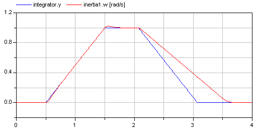
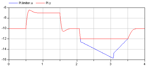
In the upper figure the reference speed (= integrator.y) and the actual speed (= inertia1.w) are shown. As can be seen, the system initializes in steady state, since no transients are present. The inertia follows the reference speed quite good until the end of the constant speed phase. Then there is a deviation. In the lower figure the reason can be seen: The output of the controller (PI.y) is in its limits. The anti-windup compensation works reasonably, since the input to the limiter (PI.limiter.u) is forced back to its limit after a transient phase.

Extends from Modelica.​Icons.​Example (Icon for runnable examples).

Parameters

Model Modelica.​Blocks.​Examples.​Filter
Demonstrates the Continuous.Filter block with various options

Information

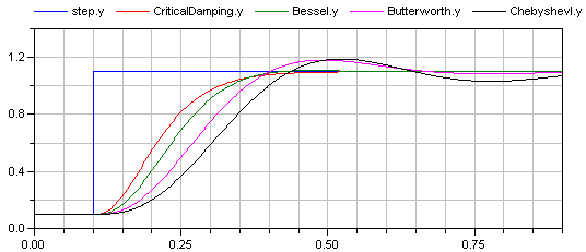
This example demonstrates various options of the Filter block. A step input starts at 0.1 s with an offset of 0.1, in order to demonstrate the initialization options. This step input drives 4 filter blocks that have identical parameters, with the only exception of the used analog filter type (CriticalDamping, Bessel, Butterworth, Chebyshev of type I). All the main options can be set via parameters and are then applied to all the 4 filters. The default setting uses low pass filters of order 3 with a cut-off frequency of 2 Hz resulting in the following outputs:

Extends from Modelica.​Icons.​Example (Icon for runnable examples).

Parameters

Model Modelica.​Blocks.​Examples.​FilterWithDifferentiation
Demonstrates the use of low pass filters to determine derivatives of filters

Information

This example demonstrates that the output of the Filter block can be differentiated up to the order of the filter. This feature can be used in order to make an inverse model realizable or to "smooth" a potential discontinuous control signal.

Extends from Modelica.​Icons.​Example (Icon for runnable examples).

Parameters

Model Modelica.​Blocks.​Examples.​FilterWithRiseTime
Demonstrates to use the rise time instead of the cut-off frequency to define a filter

Information

Filters are usually parameterized with the cut-off frequency. Sometimes, it is more meaningful to parameterize a filter with its rise time, i.e., the time it needs until the output reaches the end value of a step input. This is performed with the formula:

f_cut = fac/(2*pi*riseTime);

where "fac" is typically 3, 4, or 5. The following image shows the results of a simulation of this example model (riseTime = 2 s, fac=3, 4, and 5):

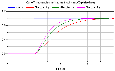
Since the step starts at 1 s, and the rise time is 2 s, the filter output y shall reach the value of 1 after 1+2=3 s. Depending on the factor "fac" this is reached with different precisions. This is summarized in the following table:

Filter order	Factor fac	Percentage of step value reached after rise time
1	3	95.1 %
1	4	98.2 %
1	5	99.3 %
2	3	94.7 %
2	4	98.6 %
2	5	99.6 %

Extends from Modelica.​Icons.​Example (Icon for runnable examples).

Parameters

Model Modelica.​Blocks.​Examples.​SlewRateLimiter
Demonstrate usage of Nonlinear.SlewRateLimiter

Information

This example demonstrates how to use the Nonlinear.SlewRateLimiter block to limit a position step with regards to velocity and acceleration:

• The Sources.Step block positionStep demands an unphysical position step.
• The first SlewRateLimiter block limit_v limits velocity.
• The first Der block v calculates velocity from the smoothed position signal.
• The second SlewRateLimiter block limit_a limits acceleration of the smoothed velocity signal.
• The second Der block a calculates acceleration from the smoothed velocity signal.
• The Integrator block positionSmoothed calculates smoothed position from the smoothed velocity signal.

A position controlled drive with limited velocity and limited acceleration (i.e. torque) is able to follow the smoothed reference position.

Extends from Modelica.​Icons.​Example (Icon for runnable examples).

Parameters

Model Modelica.​Blocks.​Examples.​InverseModel
Demonstrates the construction of an inverse model

Information

This example demonstrates how to construct an inverse model in Modelica (for more details see Looye, Thümmel, Kurze, Otter, Bals: Nonlinear Inverse Models for Control).

For a linear, single input, single output system

   y = n(s)/d(s) * u   // plant model

the inverse model is derived by simply exchanging the numerator and the denominator polynomial:

   u = d(s)/n(s) * y   // inverse plant model

If the denominator polynomial d(s) has a higher degree as the numerator polynomial n(s) (which is usually the case for plant models), then the inverse model is no longer proper, i.e., it is not causal. To avoid this, an approximate inverse model is constructed by adding a sufficient number of poles to the denominator of the inverse model. This can be interpreted as filtering the desired output signal y:

   u = d(s)/(n(s)*f(s)) * y  // inverse plant model with filtered y

With Modelica it is in principal possible to construct inverse models not only for linear but also for non-linear models and in particular for every Modelica model. The basic construction mechanism is explained at hand of this example:

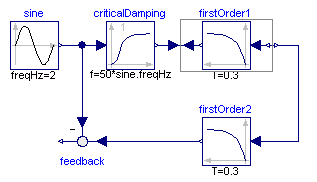
Here the first order block "firstOrder1" shall be inverted. This is performed by connecting its inputs and outputs with an instance of block Modelica.Blocks.Math.InverseBlockConstraints. By this connection, the inputs and outputs are exchanged. The goal is to compute the input of the "firstOrder1" block so that its output follows a given sine signal. For this, the sine signal "sin" is first filtered with a "CriticalDamping" filter of order 1 and then the output of this filter is connected to the output of the "firstOrder1" block (via the InverseBlockConstraints block, since 2 outputs cannot be connected directly together in a block diagram).

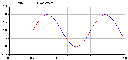
In order to check the inversion, the computed input of "firstOrder1" is used as input in an identical block "firstOrder2". The output of "firstOrder2" should be the given "sine" function. The difference is constructed with the "feedback" block. Since the "sine" function is filtered, one cannot expect that this difference is zero. The higher the cut-off frequency of the filter, the closer is the agreement. A typical simulation result is shown in the next figure:

Extends from Modelica.​Icons.​Example (Icon for runnable examples).

Model Modelica.​Blocks.​Examples.​ShowLogicalSources
Demonstrates the usage of logical sources together with their diagram animation

Information

This simple example demonstrates the logical sources in Modelica.Blocks.Sources and demonstrate their diagram animation (see "small circle" close to the output connector). The "booleanExpression" source shows how a logical expression can be defined in its parameter menu referring to variables available on this level of the model.

Extends from Modelica.​Icons.​Example (Icon for runnable examples).

Model Modelica.​Blocks.​Examples.​LogicalNetwork1
Demonstrates the usage of logical blocks

Information

This example demonstrates a network of logical blocks. Note, that the Boolean values of the input and output signals are visualized in the diagram animation, by the small "circles" close to the connectors. If a "circle" is "white", the signal is false. It a "circle" is "green", the signal is true.

Extends from Modelica.​Icons.​Example (Icon for runnable examples).

Model Modelica.​Blocks.​Examples.​RealNetwork1
Demonstrates the usage of blocks from Modelica.Blocks.Math

Information

This example demonstrates a network of mathematical Real blocks. from package Modelica.Blocks.Math. Note, that

• at the right side of the model, several Math.ShowValue blocks are present, that visualize the actual value of the respective Real signal in a diagram animation.
• the Boolean values of the input and output signals are visualized in the diagram animation, by the small "circles" close to the connectors. If a "circle" is "white", the signal is false. If a "circle" is "green", the signal is true.

Extends from Modelica.​Icons.​Example (Icon for runnable examples).

Model Modelica.​Blocks.​Examples.​IntegerNetwork1
Demonstrates the usage of blocks from Modelica.Blocks.MathInteger

Information

This example demonstrates a network of Integer blocks. from package Modelica.Blocks.MathInteger. Note, that

• at the right side of the model, several MathInteger.ShowValue blocks are present, that visualize the actual value of the respective Integer signal in a diagram animation.
• the Boolean values of the input and output signals are visualized in the diagram animation, by the small "circles" close to the connectors. If a "circle" is "white", the signal is false. If a "circle" is "green", the signal is true.

Extends from Modelica.​Icons.​Example (Icon for runnable examples).

Model Modelica.​Blocks.​Examples.​BooleanNetwork1
Demonstrates the usage of blocks from Modelica.Blocks.MathBoolean

Information

This example demonstrates a network of Boolean blocks from package Modelica.Blocks.MathBoolean. Note, that

• at the right side of the model, several MathBoolean.ShowValue blocks are present, that visualize the actual value of the respective Boolean signal in a diagram animation ("green" means "true").
• the Boolean values of the input and output signals are visualized in the diagram animation, by the small "circles" close to the connectors. If a "circle" is "white", the signal is false. If a "circle" is "green", the signal is true.

Extends from Modelica.​Icons.​Example (Icon for runnable examples).

Model Modelica.​Blocks.​Examples.​Interaction1
Demonstrates the usage of blocks from Modelica.Blocks.Interaction.Show

Information

This example demonstrates a network of blocks from package Modelica.Blocks.Interaction to show how diagram animations can be constructed.

Extends from Modelica.​Icons.​Example (Icon for runnable examples).

Model Modelica.​Blocks.​Examples.​BusUsage
Demonstrates the usage of a signal bus

Information

Signal bus concept

In technical systems, such as vehicles, robots or satellites, many signals are exchanged between components. In a simulation system, these signals are usually modelled by signal connections of input/output blocks. Unfortunately, the signal connection structure may become very complicated, especially for hierarchical models.

The same is also true for real technical systems. To reduce complexity and get higher flexibility, many technical systems use data buses to exchange data between components. For the same reasons, it is often better to use a "signal bus" concept also in a Modelica model. This is demonstrated at hand of this model (Modelica.Blocks.Examples.BusUsage):

• Connector instance "controlBus" is a hierarchical connector that is used to exchange signals between different components. It is defined as "expandable connector" in order that no central definition of the connector is needed but is automatically constructed by the signals connected to it (see also Modelica specification 2.2.1).
• Input/output signals can be directly connected to the "controlBus".
• A component, such as "part", can be directly connected to the "controlBus", provided it has also a bus connector, or the "part" connector is a sub-connector contained in the "controlBus".

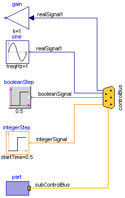
The control and sub-control bus icons are provided within Modelica.Icons. In Modelica.Blocks.Examples.BusUsage_Utilities.Interfaces the buses for this example are defined. Both the "ControlBus" and the "SubControlBus" are expandable connectors that do not define any variable. For example, Interfaces.ControlBus is defined as:

  expandable connector ControlBus
      extends Modelica.Icons.ControlBus;
      annotation ();
  end ControlBus;

Note, the "annotation" in the connector is important since the color and thickness of a connector line are taken from the first line element in the icon annotation of a connector class. Above, a small rectangle in the color of the bus is defined (and therefore this rectangle is not visible). As a result, when connecting from an instance of this connector to another connector instance, the connecting line has the color of the "ControlBus" with double width (due to "thickness=0.5").

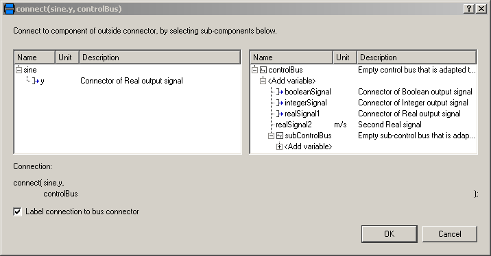
An expandable connector is a connector where the content of the connector is constructed by the variables connected to instances of this connector. For example, if "sine.y" is connected to the "controlBus", a pop-up menu may appear:

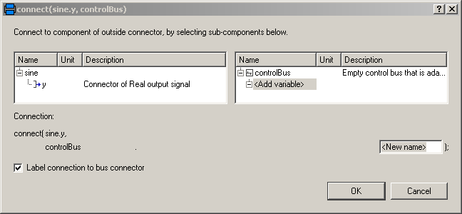
The "Add variable/New name" field allows the user to define the name of the signal on the "controlBus". When typing "realSignal1" as "New name", a connection of the form:

     connect(sine.y, controlBus.realSignal1)

is generated and the "controlBus" contains the new signal "realSignal1". Modelica tools may give more support in order to list potential signals for a connection. Therefore, in BusUsage_Utilities.Interfaces the expected implementation of the "ControlBus" and of the "SubControlBus" are given. For example "Internal.ControlBus" is defined as:

  expandable connector StandardControlBus
    extends BusUsage_Utilities.Interfaces.ControlBus;

    import SI = Modelica.SIunits;
    SI.AngularVelocity    realSignal1   "First Real signal";
    SI.Velocity           realSignal2   "Second Real signal";
    Integer               integerSignal "Integer signal";
    Boolean               booleanSignal "Boolean signal";
    StandardSubControlBus subControlBus "Combined signal";
  end StandardControlBus;

Consequently, when connecting now from "sine.y" to "controlBus", the menu looks differently:

Note, even if the signals from "Internal.StandardControlBus" are listed, these are just potential signals. The user might still add different signal names.

Extends from Modelica.​Icons.​Example (Icon for runnable examples).

Model Modelica.​Blocks.​Examples.​Rectifier6pulseFFT
Example of FFT block

Information

This example is based on a 6-pulse rectifier example, calculating the harmonics with the FFT block.

As expected, one can see the 5^th, 7^th, 11^th, 13^th, 17^th, 19^th, 23^th, 25^th, ... harmonic in the result.

Extends from Modelica.​Electrical.​Machines.​Examples.​Transformers.​Rectifier6pulse (6-pulse rectifier with 1 transformer).

Parameters

Model Modelica.​Blocks.​Examples.​Rectifier12pulseFFT
Example of FFT block

Information

This example is based on a 12-pulse rectifier example, calculating the harmonics with the FFT block.

As expected, one can see the 11^th, 13^th, 23^th, 25^th, ... harmonic in the result.

Extends from Modelica.​Electrical.​Machines.​Examples.​Transformers.​Rectifier12pulse (12-pulse rectifier with 2 transformers).

Parameters

Model Modelica.​Blocks.​Examples.​TotalHarmonicDistortion
Calculation of total harmonic distortion of voltage

Information

This example compares the result of the total harmonic distortion (THD) with respect to the fundamental wave and with respect to the total root mean square (RMS). In this simulation model a non-sinusoidal voltage wave form is created by the superposition two voltage waves:

• Fundamental wave with RMS voltage V1 and frequency f1
• Third harmonic wave with RMS voltage V3 and frequency 3*f1

This simulation model compares numerically determined THD values with results, obtained by theoretical calculations:

• Compare the numerically determined THD value thd1.y and the theoretical value THD1, both with respect to the fundamental wave; also plot thd1.valid
• Compare the numerically determined THD value thdRMS.y and the theoretical value THDrms, both with respect to the RMS value; also plot thdRMS.valid

Extends from Modelica.​Icons.​Example (Icon for runnable examples).

Parameters