Example 3
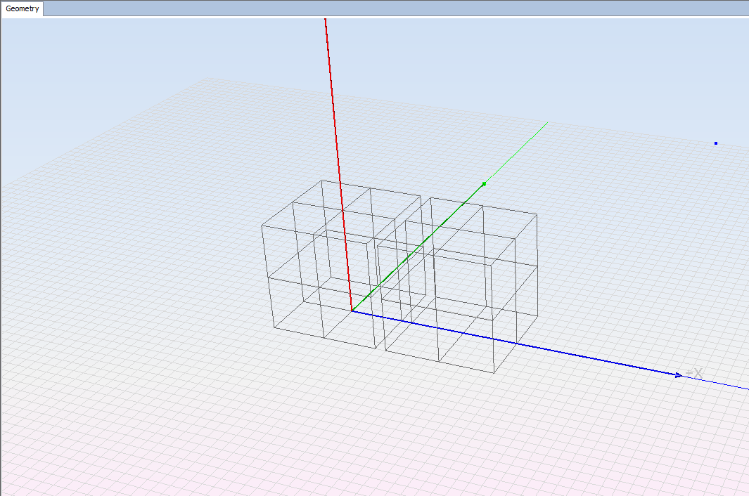
This example shows the dynamic monostatic RCS of two cubes.
Step 1
Create a new newFASANT project (using the MONCROS module) following the Step 1 to Step 3 in Example 1.
Step 2
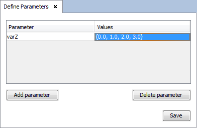
Select Geometry → Parameters→ Define parameters and introduce the following parameters.
Step 3
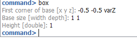
Select Geometry → Solid→ Box to define the box parameters as follows:
Step 4
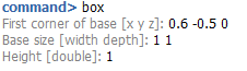
Repeat Step 3 to define another box.
Step 5
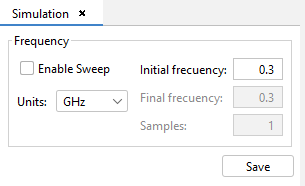
In the Simulation panel select a frequency of 0.3 GHz (default options) and press Save.
Step 6
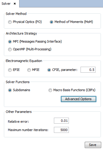
Select the Solver → Parameters option and choose CFIE solution
Step 7
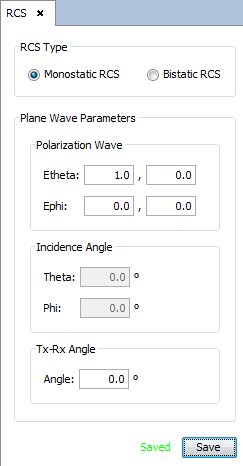
Select the RCS → Parameters option. Select Monostatic RCS and leave the default parameters. Press the Save button.
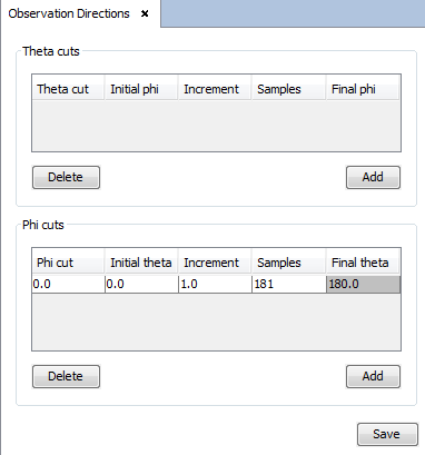
Step 8
Select Output → Observation directions. Leave the default observation directions (0.0 phi cut with theta angle varying between 0.0 and 180.0 using 181 samples).
Step 9
Before running the simulation, select the Meshing → Create Mesh option. Set 10 divisions on planar and curved surfaces, set Processors to 2 and the default number of bands per octave. Press the Mesh button.
Step 10
Select Calculate → Execute and set the number of desired processors to run the simulation. Press the Execute button to start the calculation.
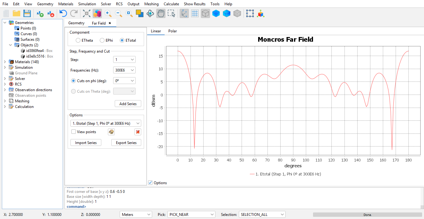
Step 11
Select Show Results → Far Field→ View Cuts to visualize the far field values for the first step.
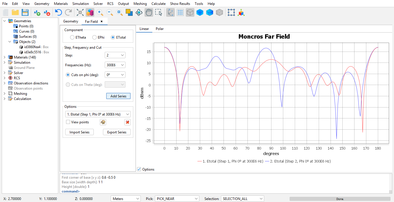
Step 12
Add a new series selecting the step on the combo box and click on Add Series button.
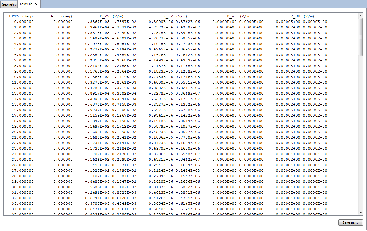
Step 13
Select Show Results → Far Field→ View Text Files to visualize the text file with the results of the simulation.