Results Module#

Result Objects#

msolve has special classes and methods to extract and store the results of a simulation. These objects provide a practical and convenient platform for post-processing.

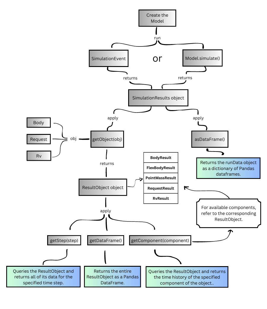
The following process map explains the different ways you can obtain the results of a simulation.

Comments

SimulationResults and SimulationResultsHistory are the classes tasked with managing the results of the simulation.

`SimulationResults`	Container object that encloses all the results from a single simulation.
`SimulationResultsHistory`	A list that can be used to store, serialize and de-serialize SimulationResults for cross plotting.

Run a SimulationEvent or use the simulate method with the returnResults attribute set to True. This instructs msolve to store the results to a SimulationResults object and return it to the caller.
Run a SimulationEvent or use the simulate method with store attribute set to True. This instructs msolve to add the SimulationResults object to a list, SimulationResultsHistory.
Use the SimulationResults.asDataFrame method to get the results as a dictionary of Pandas dataframes.

Use the SimulationResults.getObject method, specifying the entity whose results are to be extracted.

This entity can be a Body, a Request, a FrequencyInput, or a Rv.

Depending on the type of entity a ResultObject is returned. It can be one of:

`ResultObject`	Base class for all the result objects of a simulation.
`BodyResult`	Contains all the results associated with a single Part of the model.
`FrfBodyResult`	Frequency Response Simulation results for body.
`FlexBodyResult`	Contains results associated with a single FlexBody of the model.
`PointMassResult`	Contains all the results associated with a single PointMass of the model.
`RequestResult`	Contains all the results associated with a single Request of the model.
`FrfRequestResult`	Contains all the results associated with a single Request of the model for a FrequencyResponse analysis.
`FrfFrequencyResult`	Frequency Response Simulation results for FrequencyInput.
`RvResult`	Contains all the results associated with a single Rv of the model.

Use one of the methods ResultObject.getStep, ResultObject.getDataFrame, ResultObject.getComponent to extract the desired results.

Note

There is a wide range of libraries available in python for data post-processing, that can be used in conjunction with msolve.

class BodyResult#

Contains all the results associated with a single Part of the model.

At each output time, the following results are stored:

Components	Label	Index
Local Part Reference Frame (LPRF) position	X, Y, Z	0 - 2
Euler parameters	E0, E1, E2, E3	3 - 6

Example

Extract the simulation results of a Body with getComponent.#

from msolve import *

model = Model(output='body_results')

Units(system='MKS')
Accgrav(kgrav=-9.81)

ground = Part(ground=True)
global_ref = Marker(part=ground)

ball = Part(mass=1, ip=[1]*3, cm=Marker(qp=[0,0,10], zv=[0,0,1]))

run = model.simulate(type='TRANSIENT', end=2, dtout=0.01, returnResults=True)

body_results = run.getObject(ball)
#assert type(body_results) == BodyResult

time = body_results.times
ball_disp  = body_results.getComponent('Z')

import matplotlib.pyplot as plt
plt.plot(time, ball_disp)
plt.title('Vertical Displacement')
plt.xlabel('time (s)')
plt.ylabel('z (m)')
plt.grid()
plt.show()

class FlexBodyResult#

Contains results associated with a single FlexBody of the model.

At each output time, the following results are stored:

Components	Label	Index
Center of mass position	X, Y, Z	0 - 2
Euler parameters	E0, E1, E2, E3	3 - 6
Center of mass velocities	VX, VY, VZ, WX, WY, WZ	7 - 12
Center of mass accelerations	ACCX, ACCY, ACCZ, WDTX, WDTY, WDTZ	13 - 18
Modal participation factors	Q1, …. , QN	19 - (18+nmodes)
Strain Energy	SE	19+nmodes

Example

For this example, a mtx file is required. The file is located in the mbd_modeling\flexbodies folder in the MotionSolve tutorials Model Files. You may copy the file to your working directory.

Extract the simulation results of a FlexBody with asDataFrame().#

from msolve import *

model = Model(output='flex_results')

ground = Part(ground=True)
global_ref = Marker(part=ground)
Units(system='MKS')
Accgrav(kgrav=-9.81)

flex = FlexBody(mtx_file="sla_flex_left.mtx", qg=[0,0,4])
flex_marker = Marker(flex_body=flex, qp=flex.qg, zv=[0,0,1])

vel_request = Request(type="VELOCITY", i=flex_marker, j=global_ref)

run = model.simulate (type="DYNAMIC", end=0.5, steps=500, returnResults=True)

results_dict = run.asDataFrame()
print(results_dict.keys())

flex_df        = results_dict[flex]
vel_request_df = results_dict[vel_request]
print(vel_request_df.columns)

import matplotlib.pyplot as plt
plt.plot(flex_df['Z'], label="flex cm z-displacement")
plt.plot(abs(vel_request_df['VZ']), label="flex lprf z-velocity")
plt.xlabel('time (s)')
plt.legend()
plt.grid()
plt.show()

class FrfBodyResult#

Frequency Response Simulation results for body.: Contains all the results associated with a single Part of the model in a FrequencyResponse simulation for Rigid, Flexible and PointMass bodies.

When performing a Frequency Response Analysis, at each output step, the following results are stored:

Components	Label	Index
Local Part Reference Frame Results	X_MAG, X_PHASE, Y_MAG, Y_PHASE, Z_MAG, Z_PHASE	0 - 5

class FrfFrequencyResult(**kwds)#

Frequency Response Simulation results for FrequencyInput.: Contains reaction force magnitude and phase for a FrequencyInput element. Valid only for DISPLACEMENT, VELOCITY and ACCELERATION type.

When performing a Frequency Response Analysis, at each output time, the following results are stored:

Components	Label	Index
Frequency Input Reaction Force	F_MAG, F_PHASE	0 - 1

class FrfRequestResult(**kwds)#

Contains all the results associated with a single Request of the model for a FrequencyResponse analysis.

When performing a Frequency Response Analysis, at each output time, the following results are stored:

Components	Label	Index
Displacement Request	X_MAG, X_PHASE, Y_MAG, Y_PHASE, Z_MAG, Z_PHASE, B1_MAG, B1_PHASE, B2_MAG, B2_PHASE, B3_MAG, B3_PHASE	0 - 11
Velocity Request	VX_MAG, VX_PHASE, VY_MAG, VY_PHASE, VZ_MAG, VZ_PHASE, WX_MAG, WX_PHASE, WY_MAG, WY_PHASE, WZ_MAG, WZ_PHASE	0 - 11
Acceleration Request	ACCX_MAG, ACCX_PHASE, ACCY_MAG, ACCY_PHASE, ACCZ_MAG, ACCZ_PHASE, WDTX_MAG, WDTX_PHASE, WDTY_MAG, WDTY_PHASE, WDTZ_MAG, WDTZ_PHASE	0 - 11
Force Request	FX_MAG, FX_PHASE, FY_MAG, FY_PHASE, FZ_MAG, FZ_PHASE, TX_MAG, TX_PHASE, TY_MAG, TY_PHASE, TZ_MAG, TZ_PHASE	0 - 11
Expression Request	F1_MAG, F1_PHASE, F2_MAG, F2_PHASE, F3_MAG, F3_PHASE, F4_MAG, F4_PHASE, F5_MAG, F5_PHASE, F6_MAG, F6_PHASE, F7_MAG, F7_PHASE, F8_MAG, F8_PHASE	0 - 15

class PlottingMixin(**kwds)#

Base class for SimulationResults and SimulationResultsHistory.

Creates a scatter plot of (x, y, [z]) values.

x and y parameters can be defined as numerical vectors as well as string(s) to indicate a ‘result_name.component_name’ plot. if y is a list of strings or sequences and x is a list of the same length, then the two are zipped and each (x[i], y[i]) pair becomes one curve.

plot(x=None, y=None, z=None, plot_kwds=None, page_kwds=None, curve_kwds=None, plotting_package='matplotlib')#

Parameters:

x (str, list) – independent variable e.g. ‘TIME’, ‘request_name.X’ or a vectors of numbers
y (str, list) – y variable e.g. ‘request_name.Y’ or vector of numbers
z (str, list) – optional z variable e.g. ‘request_name.Z’ or vector of numbers for 3d plotting

Keyword Arguments:

plot_kwds (dict) –

Additional keyword arguments for plot customization:

{
    'name'  : 'My Plot',
    'legend': 'legend',
    'grid'  : True,
    'xlabel': 'str',
    'ylabel': 'str',
    'zlabel': 'str'
    'xlim'  : (0, 10)
    'ylim'  : (-100,100)
}

page_kwds (dict) –

Additional keyword arguments for page customization. Example:

{
    'name'    : 'page name',
    'layout'  : '1x1',
    'figsize' : (8, 5),
    'dpi'     : 96,
}

curve_kwds –
Additional keyword arguments for curve customization. In case multiple curves are defined on the same plot, you can specify a single value (e.g. ‘color’ : ‘blue’) to be used for all curves, or a list of values to be used one for each curve instance. Example:
```
{
    'color'         : 'blue',
    'name'          : 'curve_name',
    'lineStyle'     : ':',
    'x_axis_scaling': 'LINEAR',  # or LOG
    'y_axis_scaling': 'LINEAR'  # or LOG
}
```

Supported curve keywords#
Attribute	Supported values	Library support
name	any string	Matplotlib, Bokeh, Plotly
color	any CSS color string (e.g., ‘red’, ‘#FF0000’, ‘rgb(255,0,0)’)	Matplotlib, Bokeh, Plotly
lineStyle	-, –, :, -., solid, dashed, dotted, dashdot	Matplotlib, Bokeh, Plotly
marker	‘.’, ‘o’, ‘s’, ‘^’, ‘x’, ‘+’	Matplotlib
markerSize	float (e.g., 6.0)	Matplotlib
markerFaceColor	any CSS color string (e.g., ‘red’, ‘#FF0000’, ‘rgb(255,0,0)’)	Matplotlib
markerEdgeColor	any CSS color string (e.g., ‘black’, ‘#000000’, ‘rgb(0,0,0)’)	Matplotlib
markerEdgeWidth	numeric (float or int)	Matplotlib
x_axis_scaling	LINEAR, LOG	Matplotlib
y_axis_scaling	LINEAR, LOG	Matplotlib
alpha	float (0.0 to 1.0)	Matplotlib

These are some of the most popular marker symbols. For a full list see the “Markers” section of the Matplotlib API reference.

class PointMassResult#

Contains all the results associated with a single PointMass of the model.

At each output time, the following results are stored:

Components	Label	Index
LPRF position	X, Y, Z	0 - 2

Example

Extract the simulation results of a PointMass with getStep().#

from msolve import *

model = Model(output='pmass_results')

Units(system='MKS')
Accgrav(kgrav=-9.81)

ground = Part(ground=True)
global_ref = Marker(part=ground)

pmass = PointMass(mass=10, cm=Marker(qp=[0,0,10], zv=[0,0,1]), vz=8.0)

run = model.simulate(type='DYNAMIC', end=2, dtout=0.01, returnResults=True)

pmass_results = run.getObject(pmass)
#assert type(pmass_results) == PointMassResult

time = pmass_results.times

import matplotlib.pyplot as plt

# loop over the number of output time steps
for i in range(1,200):
  pmass_disp  = pmass_results.getStep(i)[2]

  plt.scatter(i*0.01, pmass_disp, linewidths=1.0)

plt.title('Vertical Displacement')
plt.xlabel('time (s)')
plt.ylabel('z (m)')
plt.grid()
plt.show()

class RequestResult#

Contains all the results associated with a single Request of the model.

At each output time, the following results are stored:

Components	Label	Index
Displacement Request	DM, DX, DY, DZ, null, PSI, THETA, PHI	0 - 7
Velocity Request	VM, VX, VY, VZ, WM, WX, WY, WZ	0 - 7
Acceleration Request	ACCM, ACCX, ACCY, ACCZ, WDTM, WDTX, WDTY, WDTZ	0 - 7
Force Request	FM, FX, FY, FZ, TM, TX, TY, TZ	0 - 7
Expression Request	F1, F2, F3, F4, F5, F6, F7, F8	0 - 7

Example

Extract the simulation results of a Request with getDataFrame().#

from msolve import *

model = Model(output='request_results')

Units(system='mmks')
Accgrav(kgrav=-9.81)

ground = Part(ground=True)
global_ref = Marker(part=ground)

part = Part(mass=10, ip=[1e3]*3, cm=Marker(qp=[0,0,10], zv=[0,0,1]))

spdp = SpringDamper(type   = 'TRANSLATION',
                    i      = part.cm,
                    j      = global_ref,
                    k      = 0.05,
                    c      = 0.005,
                    force  = 50,
                    length = 10,
                    )

vel_request = Request(type='VELOCITY', i=part.cm, j=global_ref)
acc_request = Request(f1=f'ACCZ({part.cm.id},{global_ref.id})')

run1 = model.simulate(type='DYNAMIC', end=5, dtout=0.01, returnResults=True)

spdp.c = 0.05

run2 = model.simulate(type='DYNAMIC', end=8, dtout=0.01, returnResults=True)

vel_results = run1.getObject(vel_request)
acc_results = run1.getObject(acc_request)

df = vel_results.getDataFrame()
df.columns

time          = acc_results.times
acceleration  = acc_results.getComponent('F1')

import matplotlib.pyplot as plt

plt.plot(df.VZ)
plt.plot(time, acceleration)
plt.title('Part Velocity & Acceleration time-histories')
plt.legend(['Velocity', 'Acceleration'])
plt.xlabel('time (s)')
plt.grid()
plt.show()

class ResultObject#

Base class for all the result objects of a simulation. The methods of this class are the access point to the numerical data of the simulation results.

getComponent(component)#

Queries a ResultObject and returns the time history of a specific component of the object. The components can be indexed with their index number or their respective label.

The available components for each object are listed in BodyResult, FlexBodyResult, PointMassResult, RequestResult, RvResult, FrfBodyResult, FrfRequestResult, FrfFrequencyResult.

getDataFrame()#

The entire ResultObject corresponding to the owner is returned as a Pandas DataFrame. It contains all the components and uses labels as column names.

Useful Pandas DataFrame functionalities:

df.info(): Prints concise summary of the DataFrame.
df.describe(): Generates descriptive statistics for all columns including min, std, max, mean.
df[‘column_name’] or df.column_name: Returns the column with name ‘column_name’ as a pandas Series.
df.columns: Prints a pandas index corresponding to all the columns.

getStep(step=-1)#: Queries a ResultObject and returns its data for the specific time step or the closest previous step. step can be an integer or a float value corresponding to the time step.

class RvResult#

Contains all the results associated with a single Rv of the model.

At each output time, the following results are stored:

Components	Label	Index
Value of the integral of the Rv	RVAL	0
Value of the Rv	RVAL1	1

Example

Extract the simulation results of a Response variable (Rv).#

from msolve import *

model = Model(output='rv_results')

ground = Part(ground=True)
global_ref = Marker(part=ground)
Units(system='mks')
Accgrav(kgrav=-10)

part = Part(mass=100, ip=[1,1,1], cm = Marker(qp=[0,0,1]))

c = Dv (b=0.1, blimit=[0.01, 1])
spdp = SpringDamper (type="TRANSLATION", i=part.cm, j=global_ref, k=1, c=c)

rv = Rv(function=f"DZ({part.cm.id})")

run = model.simulate(type="STATIC", end=0.5, steps=20, returnResults=True, dsa='AUTO')

rv_output   = run.getObject(rv)
time     = rv_output.times
rv_rval  = rv_output.getComponent('RVAL')
rv_rval1 = rv_output.getComponent('RVAL1')

import matplotlib.pyplot as plt
plt.plot(time, rv_rval,  label="rval")
plt.plot(time, rv_rval1, label="rval1")
plt.xlabel('time (s)')
plt.legend()
plt.grid()
plt.show()

class SimulationResults#

Container object that encloses all the results from a single simulation. This object enables you to retrieve output states for Bodies, Requests and Rvs for each output time step.

There are two ways to instruct msolve to store the simulation results. In the Model.simulate method, one of the following must be set:

onOutputStep
Function that is called when the solver hits an output step. It can be used for animation and live plots.
returnResults
Boolean that if True, causes SimulationResults to be populated.

asDataFrame(start=0, end=None)#

Returns the runData object as a dictionary of Pandas dataframes. The keys of the dictionary are the objects whose results are stored.

Parameters:

start (float) – Start time value for trimming each DataFrame.
end (float) – End time value for trimming each DataFrame.

Returns:

A new dictionary where each value is the result of the ResultObject.getDataFrame method called on the original value.

getObject(obj)#

Extracts the specified results from the SimulationResults (run) container and passes them into a ResultObject object.

Parameters:: obj (Body, Request, Rv, Name) – The object whose results are to be retrieved, or the unique name given to the object.
Returns:: The ResultObject that is associated to the obj.

Note

Using the object as a lookup key is useful, so you don’t have to know the name of the object. This approach allows for convenient lookups without relying on object names.

Using the name string as a lookup key is advantageous in scenarios such as plot templates or when working with serialized data in formats like pickle files. In such cases, the model instance and its associated objects may not be directly accessible, making the use of objects impractical. Using the name string allows for reliable lookups even when the object hierarchy is not available.

serialize_json(filename=None, zip_flag=False)#

Serializes the SimulationResults resultObjects dict object to JSON. If a filename is provided, the data is written to a JSON file or a zip file based on the zip_flag.

If zip_flag is True, a temporary JSON file is created, written, and then compressed into a zip file. The temporary file is deleted after compression. If zip_flag is False, the JSON data is written directly to the specified file.

If no filename is specified, the method returns a JSON string.

serialize_pickle(filename=None, serialize_all=False)#

Pickles the SimulationResults object. If filename is specified, the data is written to a pickle file. If not, the method returns a pickle string.

If serialize_all=False, only the tagged (named) result objects will be serialized. This is done for memory saving purposes.

summary()#

Prints a rich summary tree.

The output contains results and component hierarchy extracted from this object with color-coded output for improved readability. Example:

from msolve import *
model = createDemoPendulum()
run = model.simulate(type="TRANSIENT", end=1, steps=100, returnResults=True)
run.summary()

Warning

This functionality requires the ‘rich’ library to be installed.

class SimulationResultsHistory(**kwds)#

A list that can be used to store, serialize and de-serialize SimulationResults for cross plotting. Any simulation executed with the flag store=True will append an instance of the current SimulationResults to this class. The SimulationResultsHistory is stored as part of the model.

Example

from msolve import *
model = createDemoPendulum()
# run two simulations, each will be stored.
model.simulate(type="TRANSIENT", end=1, steps=100, store=True)
model.simulate(type="TRANSIENT", end=5, steps=1000, store=True)

# print each node in the list as a Pandas DataFrame
for run in model.simulationResultsHistory:
  print(run.asDataFrame())

serialize_json(filename=None)#: Serializes the SimulationResultsHistory to JSON. If a filename is provided, the data is written to a JSON file. If not, the method returns a JSON string.

serialize_pickle(filename=None, serialize_all=False)#: Pickles the SimulationResultsHistory object. If filename is defined, the data is written to a pkl file. If not, the method returns a pickle string. If serialize_all=False, only the tagged (named) result objects will be serialized. This is done for memory saving purposes.

plot(x=None, y=None, z=None, run=None, spline=None, plot_kwds=None, page_kwds=None, curve_kwds=None)#

Generate a 2D or 3D plot from numeric data, SimulationResults, or a Spline.

You can pass raw numeric arrays, a SimulationResults/run object (or history), or a 2D/3D Spline instance. If spline is provided, its internal x/y (and optional z) arrays will be unpacked and plotted. For 3D data, a trajectory or a surface will be drawn in Matplotlib or Plotly.

Parameters:

x (array-like or str, optional) – The independent data may be a numeric sequence (list/tuple/ndarray), a string key (e.g. ‘BODY1.Fx’) to look up from run or history or ignored if spline is provided.
y (array-like or str, optional) – The dependent data may be a numeric sequence, or a list-of-lists for a 3D surface, a string key to look up from run or history or ignored if spline is provided.
z (array-like or str, optional) – The third dimension for a 3D trajectory (flat list) or ignored in a surface (nested lists). String keys look up components.
spline (Spline, optional) – A 2D or 3D Spline instance. For 2D: spline.x, spline.y are plotted as a 2D line. For 3D: spline.x, first column of spline.y as z-grid, remaining columns as y-values rendered as a surface.
run (SimulationResults, optional) – A run object containing named result components. If None and both x and y are strings, uses the model’s SimulationResultsHistory. Otherwise, numeric data go through a dummy SimulationResults.
plot_kwds (dict, optional) –
Figure‐level options
- name (str): title of the plot.
- legend (str): legend title.
- grid (bool): whether to show grid.
- xlim (tuple): limits on the horizontal axis.
- ylim (tuple): limits on the vertical axis.
- xlabel, ylabel, zlabel (str): axis labels.
page_kwds (dict, optional) –
Page/layout options
- name (str): page name.
- layout (str): subplot grid, e.g. ‘1x1’, ‘2x2’.
- figsize (tuple): figure size in inch, e.g. (4, 6)
- dpi (int): output resolution in dots per inch. Default 96.
curve_kwds (dict, optional) –
Dictionary of Curve‐level style options or a dictionary of lists corresponding to each plotted line
- color (str): line or surface color.
- name (str or list of str): curve legend entry.
- alpha (float): opacity of the plotted element (0-1).
- lineStyle, lineThickness, marker, etc.

Returns:

the generated Plot object (for further customization).

Return type:

Plot

Raises:

ValueError – if string keys don’t match available result names/components, or if no run/history is found for string‐based inputs.

Usage

plot(x="part_displ.DX", y="part_displ.DY", z="part_displ.DZ", plot_kwds={'title': 'Trajectory'})
plot(spline=Spline(x=[-10.,-8.,-6.,-4.,-2.,0.,2.,4.,6.,8.,10.],
                   y=[-400.,-320.,-240.,-160.,-80.,0.,80.,160.,240.,320.,400.]),
                   plot_kwds={'title': '2D Spline'})