Annotations#
Some examples require external input files. Before you start, please follow the link in the Example Scripts section to download the zip file with model and result files.
Example 01 - Notes attached to Entities#
Following the standard steps (setting up the window, loading the model/result files, and contouring the results), the code defines the noteDict dictionary that contains the information used to create the notes. Specifically, it defines a list of element IDs, a list of font sizes, and a list of colors.
Next, the code loops over the lists in the noteDict dictionary and creates four notes, each attached to a different element, using a different font size and color. Finally, the latest note object is used to extract the field dictionary using getFieldDictionary() method and print out the content.
 1import hw
 2import hw.hv as hv
 3import os
 4
 5scriptDir = os.path.abspath(os.path.dirname(__file__))
 6modelFile = os.path.join(scriptDir, "aerobox", "aerobox.fem")
 7resultFile = os.path.join(scriptDir, "aerobox", "aerobox-LC1-2.op2")
 8
 9ses = hw.Session()
10ses.new()
11win = ses.get(hw.Window)
12win.type = "animation"
13
14win.addModelAndResult(modelFile, result=resultFile)
15res = ses.get(hv.Result)
16resScalar = hv.ResultDefinitionScalar(
17    dataType="Composite Stress",
18    dataComponent="vonMises",
19    layer="Max"
20)
21res.plot(resScalar)
22animTool = hw.AnimationTool()
23animTool.currentFrame = 1
24hw.evalHWC("view orientation iso")
25
26noteDict = {
27    "elements": [493, 353, 674, 733],
28    "fontSizes": [16, 12, 12, 12],
29    "colors": ["#FF0000", "#FFFFFF", "#FFFFFF", "#FFFFFF"],
30}
31
32for elem, fsize, col in zip(
33    noteDict.get("elements"), noteDict.get("fontSizes"), noteDict.get("colors")
34):
35    n = hv.Note(
36        label="Element " + str(elem),
37        attachmentType="element",
38        attachment=[1, "element", elem],
39        text="Element: {entity.id}\nValue = {entity.contour_val}",
40        textColorMode="user",
41        textColor=col,
42        borderColorMode="user",
43        borderColor=(20, 20, 20),
44        fillColor=(31, 73, 125),
45        fontSize=fsize,
46        transparency=False,
47        moveToEntity=True,
48        screenAnchor=False,
49    )
50
51fieldDic = n.getFieldDictionary()
52for key in list(fieldDic.keys()):
53    print("{:35s} {:3s} {:50s}".format(key, " = ", fieldDic[key]))
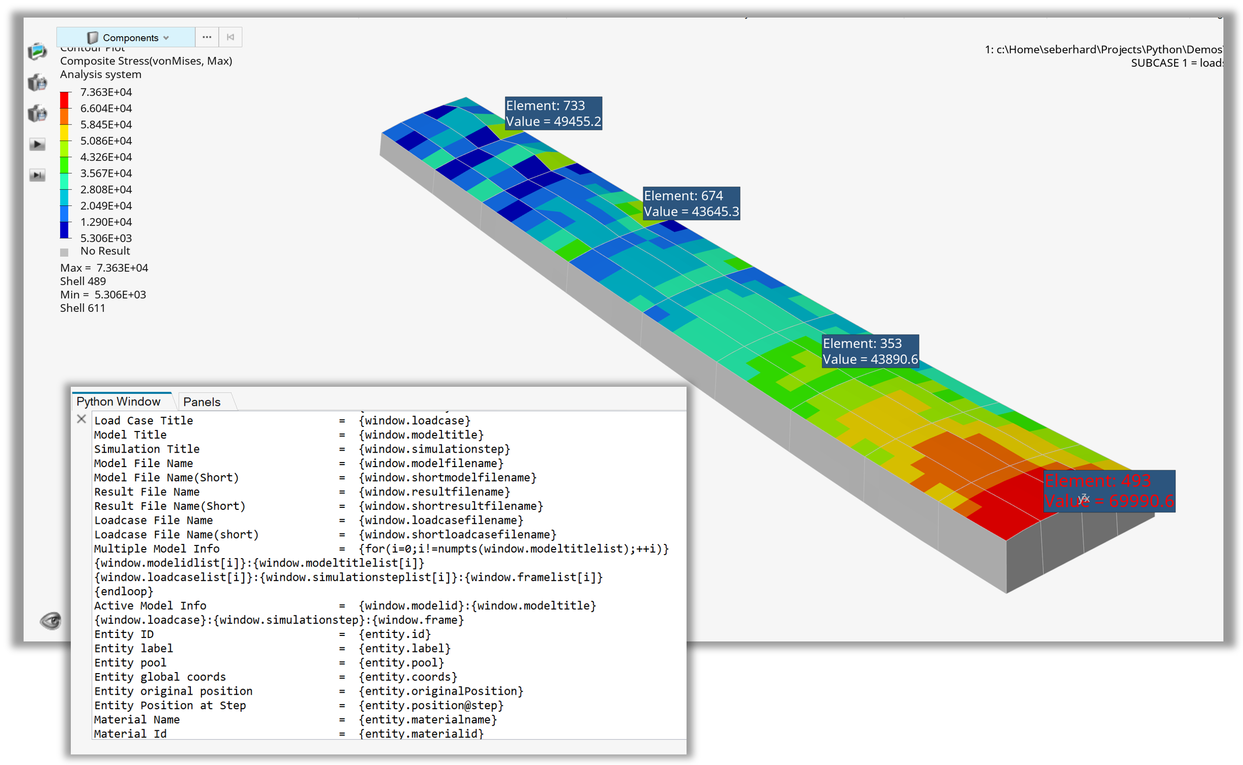
Figure 1. Notes attached to entities with getFieldDictionary() output
Example 02 - Measure Position#
After the standard steps (setting up the window, loading the model/result files, and contouring the results), the code sets the model orientation using the HWC view command and creates objects n1, n2, and n3 for nodes ID 207, 11, and 44 respectively. These three nodes are used to create a new rectangular system (sysRect) that will be assigned to the MeasurePosition entity.
Next, a list of node objects (nodeObjectList) is created for nodes ID 1075, 999, 1568, and 1266. At this point, all the required variables are defined and a new MeasurePosition is created. The node objects are assigned to it via the addEntities() method and the system attribute is set to sysRect.
 1import hw
 2import hw.hv as hv
 3import os
 4
 5ALTAIR_HOME = os.path.abspath(os.environ['ALTAIR_HOME'])
 6modelFile   = os.path.join(ALTAIR_HOME,'demos','mv_hv_hg','animation','dyna','bumper','bumper_deck.key')
 7resultFile  = os.path.join(ALTAIR_HOME,'demos','mv_hv_hg','animation','dyna','bumper','d3plot')
 8
 9ses = hw.Session()
10ses.new()
11win=ses.get(hw.Window)
12win.type = 'animation'
13
14win.addModelAndResult(modelFile, result=resultFile)
15res = ses.get(hv.Result)
16resScalar = hv.ResultDefinitionScalar(dataType='Displacement',
17                dataComponent='Mag')
18res.plot(resScalar)
19animTool = hw.AnimationTool()
20animTool.currentFrame=26
21
22hw.evalHWC('view projection orthographic | \
23         view matrix  0.174593   0.948911    0.262841 \
24                 0.000000  -0.964156    0.218925 \
25                -0.149918   0.000000   -0.199801 \
26                -0.227245   0.953121    0.000000 \
27                 351.268646 512.829834 -658.386963 1.000000 | \
28         view clippingregion -251.830444  96.738075  555.359558 \
29                837.470154 -722.333801 601.748169')
30
31model  = ses.get(hv.Model)
32n1 = model.get(hv.Node,207)
33n2 = model.get(hv.Node,11)
34n3 = model.get(hv.Node,44)
35
36sysRect = hv.System(type='rectangular',fixed=False)
37sysRect.label = 'Rectangular System'
38sysRect.labelVisibility = True
39sysRect.setOrientationByNode(
40            origin     = n1,
41            axis       = n2,
42            plane      = n3,
43            axisplane  = 'X-XY'
44)
45
46nodeIdList = [1075,999,1568,1266]
47nodeObjectList = [ model.get(hv.Node,id) for id in nodeIdList ]
48
49measurePosition = hv.MeasurePosition()
50
51measurePosition.addEntities(nodeObjectList)
52measurePosition.label               = 'Position'
53measurePosition.displayLabel        = True
54measurePosition.displayId           = True
55measurePosition.color               = (0,0,0)
56measurePosition.fontSize            = 12
57measurePosition.numericFormat       = 'scientific'
58measurePosition.numericPrecision    = 3
59measurePosition.transparency        = False
60measurePosition.autohide            = True
61measurePosition.prefix              = True
62measurePosition.system              = sysRect
63
64win.draw()
65print(measurePosition.getMeasureProperties())
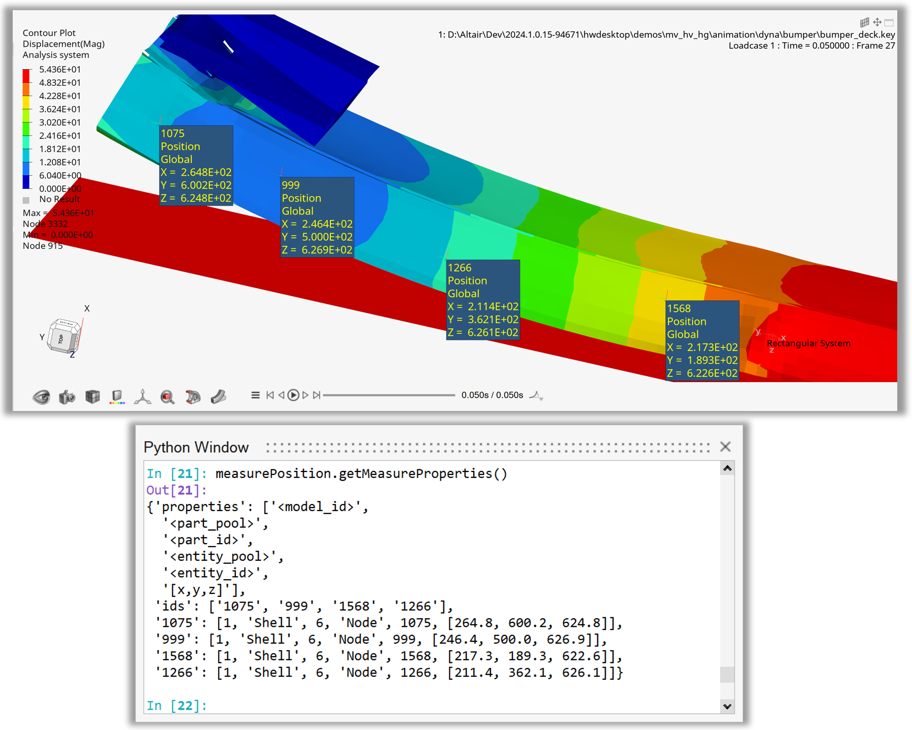
Figure 2. Position measures using node id list and print measure properties
Example 03 - Measure Minimum Distance#
After the standard steps (setting up the window, loading the model/result files, and contouring the results), the code sets the model orientation using the HWC view command and creates objects n1, n2, and n3 for nodes ID 207, 11, and 44 respectively. These three nodes are used to create a new rectangular system (sysRect) that will be assigned to the MeasurePosition entity.
Next, three collections are created. col1 is a node collection populated with nodes from component ID 3 using the addByID() method. col2 is a component collection populated with component named “Mounting Bracket” using the addByComponentName() method. col3 is a component collection populated with components that include the nodes from col1, i.e. it includes component ID 3.
Subsequently, a new collection colHide is created by combining col2 and col3 using simple arithmetics on the collection objects. All other components in the model are then hidden and a new MeasureDistanceMinimum object is created to measure the minimum distance between entities in col1 and col2. The collections are assigned to to the measure object via the addEntities() method and the system attribute is set to sysRect.
Note
In HyperView, the component entity is represented by the Part class.
 1import hw
 2import hw.hv as hv
 3import os
 4
 5ALTAIR_HOME = os.path.abspath(os.environ['ALTAIR_HOME'])
 6modelFile   = os.path.join(ALTAIR_HOME,'demos','mv_hv_hg','animation','dyna','bumper','bumper_deck.key')
 7resultFile  = os.path.join(ALTAIR_HOME,'demos','mv_hv_hg','animation','dyna','bumper','d3plot')
 8
 9ses = hw.Session()
10ses.new()
11win=ses.get(hw.Window)
12win.type = 'animation'
13
14win.addModelAndResult(modelFile, result=resultFile)
15res = ses.get(hv.Result)
16resScalar = hv.ResultDefinitionScalar(dataType='Displacement',
17                dataComponent='Mag')
18res.plot(resScalar)
19animTool = hw.AnimationTool()
20animTool.currentFrame=26
21
22
23hw.evalHWC('view projection orthographic | \
24         view matrix  0.429744 0.751905 0.499958 \
25                 0.000000 -0.469094 0.659022 \
26                -0.587913 0.000000 -0.771538 \
27                 0.018125 0.635925 0.000000 \
28                 460.527435 157.489700 -354.629974 1.000000 | \
29          view clippingregion -251.830444 96.738075 555.359558 \
30                837.470154 -722.333801 601.748169')
31
32model  = ses.get(hv.Model)
33n1 = model.get(hv.Node,207)
34n2 = model.get(hv.Node,11)
35n3 = model.get(hv.Node,44)
36
37sysRect = hv.System(type='rectangular',fixed=False)
38sysRect.label = 'Rectangular System'
39sysRect.labelVisibility = True
40sysRect.setOrientationByNode(
41            origin = n1,
42            axis       = n2,
43            plane      = n3,
44            axisplane  = 'X-XY'
45)
46
47col1 = hv.Collection(hv.Node,populate=False)
48col1.addByID(hv.Part,3)
49
50col2 = hv.Collection(hv.Part,populate=False)
51col2.addByComponentName(['Mounting Bracket'])
52
53col3 = hv.Collection(hv.Part,populate=False)
54col3.addByID(hv.Node,col1.getIds())
55
56colHide = col2 + col3
57[p.setAttributes(meshMode='shadedMeshLines') for p in  colHide.getEntities()]
58colHide.reverse()
59model.hide(colHide)
60
61measureDistanceMinimum = hv.MeasureDistanceMinimum()
62measureDistanceMinimum.addEntities(col1,col2)
63
64measureDistanceMinimum.label               = 'Minimum Distance'
65measureDistanceMinimum.displayLabel        = True
66measureDistanceMinimum.displayId           = True
67measureDistanceMinimum.color               = '#000000'
68measureDistanceMinimum.fontSize            = 12
69measureDistanceMinimum.numericFormat       = 'fixed'
70measureDistanceMinimum.numericPrecision    = 3
71measureDistanceMinimum.transparency        = False
72measureDistanceMinimum.autohide            = False
73measureDistanceMinimum.prefix              = True
74measureDistanceMinimum.system              = sysRect
75
76win.draw()
77print(measureDistanceMinimum.getMeasureProperties())
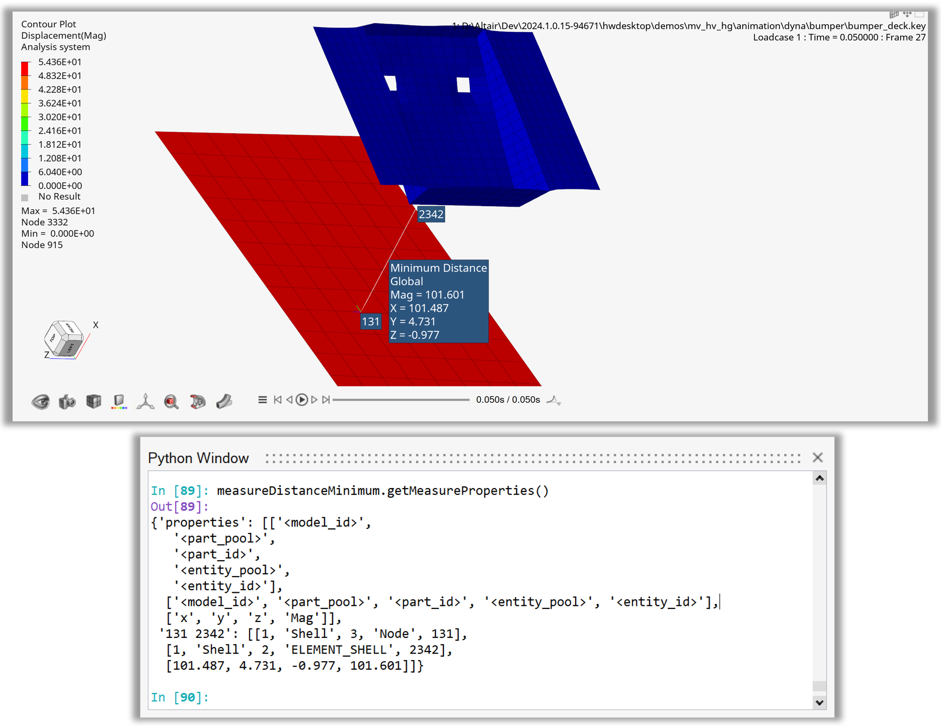
Figure 3. Minimum distance measure between between node and part collections
Example 04 - Hotspot with Defaults#
After loading the model and contouring Stress – von Mises, the animation tool is used to set the display to the last timestep.
A new hotspot object is then created with default values.
Using the hotspot.find() and hotspot.review() methods, the hotspots are displayed in the animation window.
Note
In HyperView, the hotspot entity is represented by the Hotspot class.
 1    import hw
 2    import hw.hv as hv
 3    import os
 4
 5    scriptDir   = os.path.abspath(os.path.dirname(__file__)).replace('\\','/')
 6    modelFile   = os.path.join(scriptDir,'.','truck','truck.key').replace('\\','/')
 7    resultFile  = os.path.join(scriptDir,'.','truck','d3plot').replace('\\','/')
 8
 9    ses = hw.Session()
10    ses.new()
11    win= ses.get(hw.Window)
12    win.type = 'animation'
13    win.addModelAndResult(modelFile, result=resultFile)
14    res = ses.get(hv.Result)
15    if ses.getMultiCoreMode():
16            res.loadAnimation(frame='all')
17    resScalar = hv.ResultDefinitionScalar(dataType='Stress',dataComponent='vonMises')
18    res.plot(resScalar,True)
19    animTool=hw.AnimationTool()
20    animTool.currentFrame=res.getSimulationIds()[-2]
21    win.draw()
22
23    hotspot = hv.Hotspot()
24    hotspot.default()
25    hotspot.label = 'Hotspot1Defaults'
26    numHotspot = hotspot.find()
27    hotspot.review()
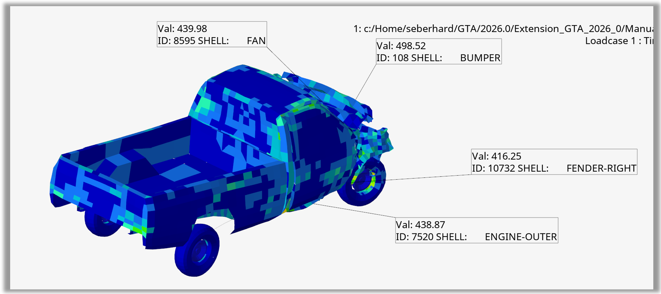
Figure 4. Hotspot with default values
Example 05 - Hotspots Global Spheres from Part Collection#
After loading the model and contouring Stress – von Mises, the animation tool is used to set the display to the last timestep.
With the hotspot object, criteria attributes such as criteriaFilterType, criteriaLowerValue, and criteriaSeparation are set.
Attributes such as hotspot.modeFocusRegion and hotspot.modeTransparency are used to control the appearance of the hotspots.
A part collection containing IDs from the front of the truck model defines the range for the hotspot search.
Using the hotspot.find() and hotspot.review() methods, the hotspots are displayed in the animation window.
Finally, the hotspot.setViewMode() method is used to set the view to Global – Sphere.
Note
In HyperView, the hotspot entity is represented by the Hotspot class.
 1    import hw
 2    import hw.hv as hv
 3    import os
 4
 5    scriptDir   = os.path.abspath(os.path.dirname(__file__)).replace('\\','/')
 6    modelFile   = os.path.join(scriptDir,'.','truck','truck.key').replace('\\','/')
 7    resultFile  = os.path.join(scriptDir,'.','truck','d3plot').replace('\\','/')
 8
 9    ses = hw.Session()
10    ses.new()
11    win= ses.get(hw.Window)
12    win.type = 'animation'
13    win.addModelAndResult(modelFile, result=resultFile)
14    res = ses.get(hv.Result)
15    if ses.getMultiCoreMode():
16            res.loadAnimation(frame='all')
17    resScalar = hv.ResultDefinitionScalar(dataType='Stress',dataComponent='vonMises')
18    res.plot(resScalar,True)
19    animTool=hw.AnimationTool()
20    animTool.currentFrame=res.getSimulationIds()[-2]
21    win.draw()
22
23    hotspot = hv.Hotspot()
24    hotspot.default()
25    hotspot.label = 'Hotspot2PartSelection'
26    hotspot.criteriaFilterType = 'greaterThan'
27    hotspot.criteriaLowerValue = 300.0
28    hotspot.criteriaSeparation = 500.0
29    hotspot.criteriaStartSeparation = 'max'
30    hotspot.criteriaLoadCase = 'current'
31    hotspot.modeFocusRegion = 'user'
32    hotspot.modeFocusRegionSize = 100
33    hotspot.modeTransparency = 0.8
34    partCol = hv.Collection(hv.Part,populate = False)
35    partCol.addByID(hv.Part,[1,  3,  4,  5,  6,  9, 10,
36                            11, 12, 13, 16, 17, 18, 19,
37                            20, 21, 31, 32, 33, 34, 35,
38                            45, 46, 47, 48, 49, 58, 60, 61])
39    print(f'Part collection Size = {partCol.getSize()}')
40    for p in partCol.getEntities():
41            print(f'    Part =  {p.id} {p.name}')
42    hotspot.criteriaSelect = partCol
43    numHotspot = hotspot.find()
44    hotspot.review()
45    hotspot.setViewMode(['global', 'sphere'])
46    win.draw()
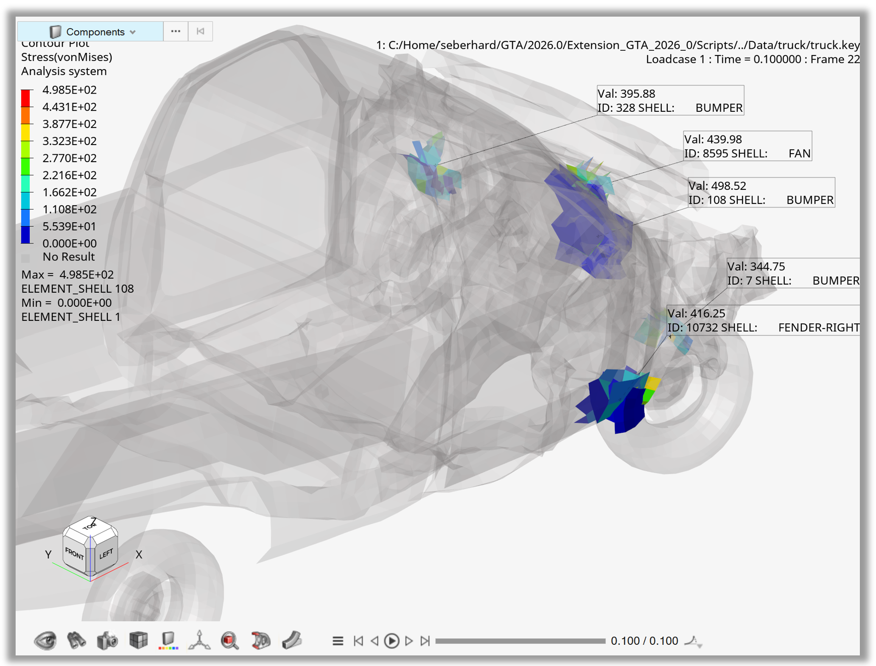
Figure 5. Hotspots with global sphere view for part collection
Example 06 - Hotspots Export Images and CSV#
After loading the model and contouring Stress – von Mises, the animation tool is used to set the display to the last timestep.
The hotspot object criteria and mode values are set, and the hotspots are displayed using the hotspot.find() and hotspot.review() methods.
The hotspot.setViewMode() method sets the view to Component – Isolate, and the hotspot.resultTableExportCSV() method exports the results to an Excel CSV file.
Finally, the script loops over all hotspots and creates one PNG image per hotspot using the hw.CaptureImageTool() in a custom size.
Note
In HyperView, the hotspot entity is represented by the Hotspot class.
 1    import hw
 2    import hw.hv as hv
 3    import os
 4    import time
 5    from pathlib import Path
 6
 7    scriptDir      = os.path.abspath(os.path.dirname(__file__)).replace('\\','/')
 8    modelFile      = os.path.join(scriptDir,'.','truck','truck.key').replace('\\','/')
 9    resultFile     = os.path.join(scriptDir,'.','truck','d3plot').replace('\\','/')
10    exportDir      = os.path.join(scriptDir,'.','Export').replace('\\','/')
11    hotspotCSVfile = os.path.join(exportDir,'resultsHotspots.csv').replace('\\','/')
12
13    ses = hw.Session()
14    ses.new()
15    win= ses.get(hw.Window)
16    win.type = 'animation'
17    win.addModelAndResult(modelFile, result=resultFile)
18    res = ses.get(hv.Result)
19    if ses.getMultiCoreMode():
20            res.loadAnimation(frame='all')
21    resScalar = hv.ResultDefinitionScalar(dataType='Stress',dataComponent='vonMises')
22    res.plot(resScalar,True)
23    animTool=hw.AnimationTool()
24    animTool.currentFrame=res.getSimulationIds()[-2]
25    win.draw()
26
27    captureTool = hw.CaptureImageTool(type = 'jpg',width = 3000,height = 2000)
28
29    hotspot = hv.Hotspot()
30    hotspot.default()
31    hotspot.label = 'Hotspot3Export'
32    hotspot.criteriaFilterType = 'greaterThan'
33    hotspot.criteriaLowerValue = 300.0
34    hotspot.criteriaSeparation = 500.0
35    hotspot.criteriaStartSeparation = 'max'
36    hotspot.criteriaLoadCase = 'current'
37    hotspot.modeFocusRegion = 'user'
38    hotspot.modeFocusRegionSize = 100
39    hotspot.modeTransparency = 0.8
40    numHotspot = hotspot.find()
41    hotspot.review()
42    hotspot.setViewMode(['component','isolate'])
43    hotspot.resultTableExportCSV(hotspotCSVfile)
44    for i in list(range(1,numHotspot+1)):
45            time.sleep(0.5)
46            hotspot.displayNext()
47            image = f'Hotspot_{i}.jpg'
48            captureTool.file = os.path.join(exportDir,image)
49            captureTool.capture()
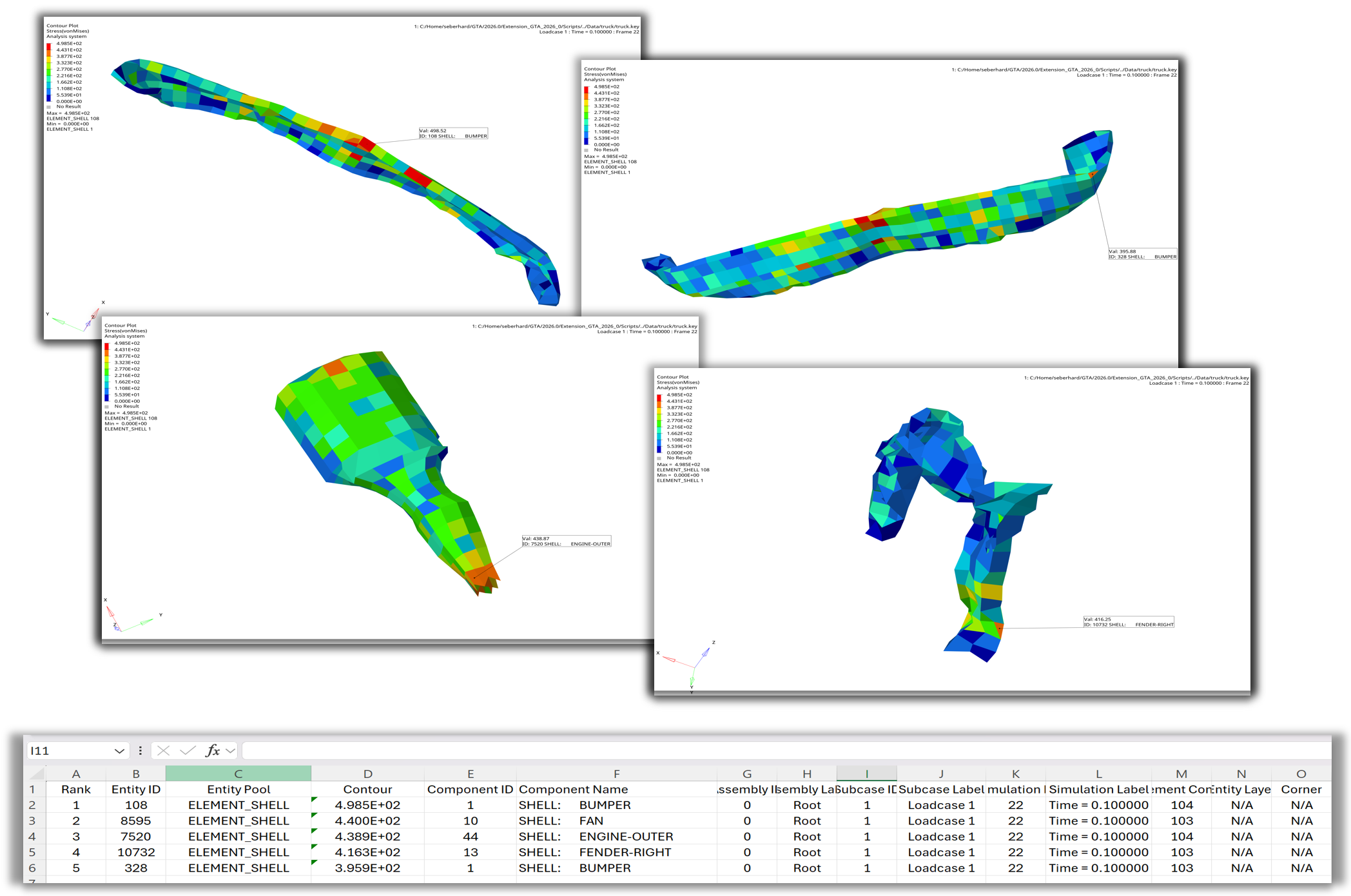
Figure 6. Loop over hotspots and export images and CSV file
Example 07 - Hotspot Measures, Notes, Sets#
After loading the model and contouring Stress – von Mises, the animation tool is used to set the display to the last timestep.
The hotspot object’s criteria values and modes are set, and the note text, location, colors, and numeric format are customized.
Using the hotspot.find() and hotspot.review() methods, the hotspots are displayed.
The hotspot.setViewMode() method sets the view to Global – Sphere.
The temporary hotspot annotations are converted to permanent notes, measures, and sets using the hotspot.createNotes(), hotspot.createMeasures(), and hotspot.createSets() methods.
Note
In HyperView, the hotspot entity is represented by the Hotspot class.
 1    import hw
 2    import hw.hv as hv
 3    import os
 4    import textwrap
 5    import pprint
 6
 7    scriptDir   = os.path.abspath(os.path.dirname(__file__)).replace('\\','/')
 8    modelFile   = os.path.join(scriptDir,'.','truck','truck.key').replace('\\','/')
 9    resultFile  = os.path.join(scriptDir,'.','truck','d3plot').replace('\\','/')
10
11    ses = hw.Session()
12    ses.new()
13    win= ses.get(hw.Window)
14    win.type = 'animation'
15    win.addModelAndResult(modelFile, result=resultFile)
16    res = ses.get(hv.Result)
17    if ses.getMultiCoreMode():
18            res.loadAnimation(frame='all')
19    resScalar = hv.ResultDefinitionScalar(dataType='Stress',dataComponent='vonMises')
20    res.plot(resScalar,True)
21    animTool=hw.AnimationTool()
22    animTool.currentFrame=res.getSimulationIds()[-2]
23    win.draw()
24
25    hotspot = hv.Hotspot()
26
27    hotspot.criteriaFilterType = 'greaterThan'
28    hotspot.criteriaLowerValue = 300.0
29    hotspot.criteriaSeparation = 500.0
30    hotspot.criteriaStartSeparation = 'max'
31    hotspot.criteriaLoadCase = 'current'
32    hotspot.criteriaNumberOfHotspotTopValue = 3
33
34    hotspot.modeFocusRegion = 'user'
35    hotspot.modeFocusRegionSize = 50
36    hotspot.modeTransparency = 0.9
37
38    hotspot.noteType =  'static'
39    hotspot.noteDistance =  0.3
40    hotspot.noteLocation = 'aboveleft'
41    hotspot.noteText = """Val: {entity.contour_val}
42    ID: {entity.id} {parent.label}
43    Top 3 Hotspots"""
44    hotspot.noteFillTransparency = False
45    hotspot.noteTextColorMode = 'contour'
46    hotspot.noteFillColorMode = 'user'
47    hotspot.noteFillColor  = (255,255,255)
48    hotspot.noteBorderColorMode = 'contour'
49    hotspot.noteBorderThickness = 2
50    hotspot.noteDisplaySpotRank = True
51    hotspot.noteNumericFormat = 'fixed'
52
53    numHotspot = hotspot.find()
54    hotspot.review()
55    hotspot.setViewMode(['global', 'sphere'])
56
57    measureList = hotspot.createMeasures()
58    print(f'Number of Measures  = {len(measureList)}')
59    for measure in measureList:
60            print(f'  - Measure "{measure.label}"')
61            pprint.pprint(measure.getMeasureProperties(), indent=4)
62    noteList = hotspot.createNotes()
63    print(f'Number of Notes  = {len(noteList)}')
64    for note in noteList:
65            print(f'  - Note "{note.label}"')
66            print(f'      noteType          = {hotspot.noteType}')
67            print(f'      noteDistance      = {hotspot.noteDistance}')
68            print(f'      noteLocation      = {hotspot.noteLocation}')
69            print(f'      noteTextColorMode = {hotspot.noteTextColorMode}')
70            print(f'      Templex Expression:')
71            print(textwrap.indent(hotspot.noteText, '        '))
72            print(f'      Templex Evaluated:')
73            print(textwrap.indent(note.textAsDisplayed, '        '))
74
75    setList = hotspot.createSets()
76    print(f'Number of Sets  = {len(setList)}')
77    for s in setList:
78            print(f'  - Set "{s.label}"')
79            print(f'        - entityType = {s.entityType}')
80            print(f'        - size       = {s.getSize()}')
81    win.fit()
82    hotspot.clear()
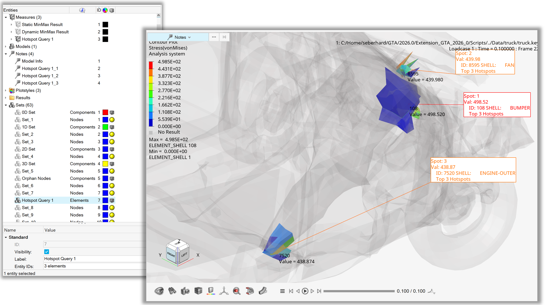
Figure 7. Hotspot - Creation of Measure Group, Notes and Set
Example 08 - Hotspot All Loadcases Simulations#
After loading the model and contouring Stress – von Mises, the animation tool is used to set the display to the last timestep.
The hotspot.criteriaSimulations() method is used to search across all load cases and simulations by using wildcards in the dictionary.
Finally, the hotspots are displayed using the hotspot.find() and hotspot.review() methods.
Note
In HyperView, the hotspot entity is represented by the Hotspot class.
 1    import hw
 2    import hw.hv as hv
 3    import os
 4
 5    scriptDir   = os.path.abspath(os.path.dirname(__file__)).replace('\\','/')
 6    modelFile   = os.path.join(scriptDir,'.','aerobox','aerobox.fem').replace('\\','/')
 7    resultFile  = os.path.join(scriptDir,'.','aerobox','aerobox-LC1-2.op2').replace('\\','/')
 8
 9    ses = hw.Session()
10    ses.new()
11    win= ses.get(hw.Window)
12    win.type = 'animation'
13    win.addModelAndResult(modelFile, result=resultFile)
14    res = ses.get(hv.Result)
15    if ses.getMultiCoreMode():
16            res.loadAnimation(frame='all')
17    resScalar = hv.ResultDefinitionScalar(dataType='Stress',dataComponent='vonMises')
18    res.plot(resScalar,True)
19
20    hotspot = hv.Hotspot()
21    hotspot.label = 'Hotspot4SubcaseMeasureNotes'
22    hotspot.criteriaFilterType = 'greaterThan'
23    hotspot.criteriaLowerValue = 1000.0
24    hotspot.criteriaSeparation = 500.0
25    hotspot.criteriaNumberOfHotspotTopValue = 3
26    inputDictionary = {'all': 'all'}
27    hotspot.criteriaSimulations = inputDictionary
28    numHotspot = hotspot.find()
29    hotspot.review()
30
31    win.fit()
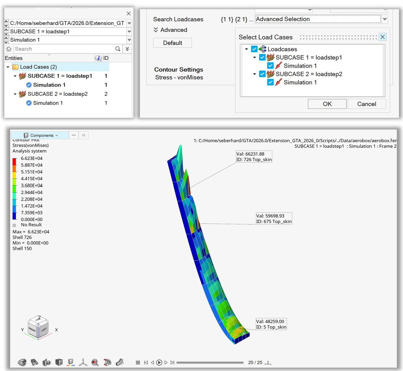
Figure 8. Hotspot from all loadcases and simulations