Inputs

Standard inputs ––––--

Modes of computation

There are two modes of computation.

The “Fast” computation mode is the default one. It corresponds to a hybrid model, which is perfectly suited for the pre-design step. Indeed, all the computations in the back end are based on magnetostatic finite element computations associated with Park’s transformation. It evaluates the electromagnetic quantities with the best compromise between accuracy and computation time to explore the space of solutions quickly and easily.

The “Accurate” computation mode allows solving the computation with transient magnetic finite element modeling. This mode of computation is perfectly suited to the final design step because it allows getting more accurate results. It also computes additional quantities like the AC losses in winding and rotor iron losses.

Current definition mode

There are 2 common ways to define the electrical current.

Electrical current can be defined by the current density in electric conductors.

In this case, the current definition mode should be « Density ».

Electrical current can be defined directly by indicating the value of the line current (the RMS value is required).

In this case, the current definition mode should be « Current ».

Field current

When the choice of current definition mode is “Current”, the DC value of the current supplied to the field winding: “Field current” (Current in Field conductors) must be provided.

Field current density

When the choice of current definition mode is “Density”, the DC value of the current density in electric conductors “Field current density” (Current density in Field conductors) must be provided.

Note: The number of parallel paths is automatically considered in the results.

Line current h1, rms

When the choice of current definition mode is “Current”, the rms value of the line current supplied to the machine: “Line current, h1 rms” (Line current, first harmonic rms value) must be provided.

Current density h1, rms

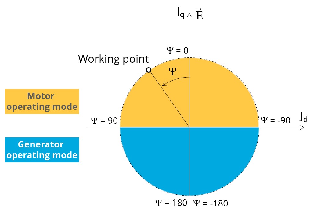
When the choice of current definition mode is “Density”, the rms value of the current density in electric conductors “Current density, h1 rms” (Current density in conductors, first harmonic rms value) must be provided.

Note: The number of parallel paths and the winding connection are automatically considered in the results.

Control angle

Considering the vector diagram shown below, the “Control angle” is the angle between the electromotive force (E) and the electrical current (J) (Ψ = angle (E, J)).

The default value is 45 degrees. It is an electrical angle. It must be set in a range of -180 to 180 degrees.

This range of values covers all the possible working points in the motor convention. The operating mode is displayed at the head of the results.

Note: The sign of results like power depends on both the convention and the operating mode.

Figure 1. Definition of the control angle Ψ - Motor convention

Speed

The imposed “Speed” (Speed) of the machine must be set.

Rotor position dependency

This input is enabled only if the “Fast” mode is selected. By default, the rotor position dependency is set to “No”, but it can be set to “Yes”.

When selected, this option allows the user to carry out the test by considering the rotor position. Hence, the computation will be done with rotor position θr varying within the “No. computed elec. periods”, providing a better estimate of machine performance while maintaining a relatively low computation time compared with “Accurate mode”.

Note: In “Fast” mode, the ripple torque is analyzed only if the “Rotor position dependency” is Yes.

AC losses analysis - Fast

The “AC losses analysis - Fast” (AC losses analysis required only while “Fast” computation mode and Rotor position dependency are selected) allows computing or not AC losses in stator winding. There are two available options:

None: AC losses are not computed. However, as the computation mode is “Fast” with rotor position dependency, a multi-static computation is performed without representing the solid conductors (wires) inside the slots. Phases are modeled with coil regions. Thus, the mesh density (number of nodes) is lower which leads to a lower computation time.

FE-Hybrid: AC losses in winding are computed without representing the wires (strands, solid conductors) inside the slots.

Since the location of each wire is accurately defined in the winding environment, sensors evaluate the evolution of the flux density close each wire. Then, a postprocessing based on analytical approaches computes the resulting current density inside the conductors and the corresponding Joule losses.

The wire topology can be “Circular” or “Rectangular”.

There can be one or several wires in parallel (in hand) in a conductor (per turn).

This method leads to quite accurate results with lower computation time. This is a good compromise between accuracy and computation time.

Warning: With the “FE-Hybrid” option the accuracy of results is good especially when the wire size is small (let’s say wire diameter lower than 2.5 mm). However, this can have a little impact on the accuracy of results because we have supposed that the magnetic field is not impacted by the modeling assumption

Note: With FE-Hybrid option the recommended “Number of computed electrical periods” is equal to “1/2”.

Note: When the winding is built with hairpin technology the FE-Hybrid mode is not available because it is not relevant for computations with such kind of winding/conductors.

AC losses analysis - Accurate

The “AC losses analysis - Accurate” (AC losses analysis required only while “Accurate” computation mode is selected) allows computing or not AC losses in stator winding. There are three options available:

None: AC losses are not computed. However, as the computation mode is “Accurate”, a transient computation is performed without representing the solid conductors (wires) inside the slots. Phases are modeled with coil regions. Thus, the mesh density (number of nodes) is lower which leads to a lower computation time.

FE-One phase: AC losses are computed with only one phase modeled with solid conductors (wires) inside the slots. The other two phases are modeled with coil regions. Thus, AC losses in winding are computed with a lower computation time than if all the phases were modeled with solid conductors. However, this can have a little impact on the accuracy of results because we have supposed that the magnetic field is not impacted by the modeling assumption.

FE-All phase: AC losses are computed, with all phases modeled with solid conductors (wires) inside the slots. This computation method gives the best results in terms of accuracy, but with a higher computation time.

FE-Hybrid: AC losses in winding are computed without representing the wires (strands, solid conductors) inside the slots.

Since the location of each wire is accurately defined in the winding environment, sensors evaluate the evolution of the flux density close each wire. Then, a postprocessing based on analytical approaches computes the resulting current density inside the conductors and the corresponding Joule losses.

The wire topology can be “Circular” or “Rectangular”.

There can be one or several wires in parallel (in hand) in a conductor (per turn).

This method leads to quite accurate results with lower computation time. This is a good compromise between accuracy and computation time.

Warning: With the “FE-Hybrid” option the accuracy of results is good especially when the wire size is small (let’s say wire diameter lower than 2.5 mm). However, this can have a little impact on the accuracy of results because we have supposed that the magnetic field is not impacted by the modeling assumption.

Note: With FE-Hybrid option the recommended “Number of computed electrical periods” is equal to “1/2” whereas 2 computed electrical periods are needed for “FE-One phase” and for “FE-All phase” options.

Indeed, when solid conductors are represented in the Finite Element model (like with FE-One phase and FE-All phase options), there are transient phenomena to consider which leads to increase the “Number of computed electrical periods” to reach the steady state.

With the “FE-Hybrid option”, the transient phenomena are handled by the analytical model, so, it is not necessary to increase the “Number of computed electrical periods” compared to a study with “None” options (without AC losses computation).

Note: When the winding is built with a hairpin technology the FE-Hybrid mode is not available because it is not relevant for computations with such kind of winding/conductors.

Advanced inputs ––––--

No. computed elec. periods

The user input “No. computed elec. periods” (Number of computed electrical periods only required with “Accurate” computation mode or “Fast” computation mode with rotor position dependency activated) influences the accuracy of results, especially in the case of AC losses computation. Indeed, with represented conductors (AC losses analysis set to “FE - One phase” or “FE - All phase”), the computation may lead to have transient current evolution in wires requiring more than an electrical period of simulation to reach the steady state over an electrical period.

The default value is equal to 2. The minimum allowed value is 0.5 (recommended in “Accurate” mode with AC losses analysis set to “None” or “Hybrid” and “Fast” mode with rotor position dependency). The default value provides a good compromise between the accuracy of results and computation time.

No. comp / elec. period

The user input “No. comp / elec. period” (Number of computations per electrical period required only with “Accurate” computation mode or “Fast” computation mode with rotor position dependency activated) influences the accuracy of results (computation of the peak-peak ripple torque, iron losses, AC losses…) and the computation time.

The default value is equal to 40. The minimum recommended value is 20. The default value provides a good balance between accuracy of results and computation time.

Skew model – No. of layers

When the rotor magnets or the stator slots are skewed, the number of layers used in Altair Flux Skew environment to model the machine can be modified: “Skew model - No. of layers” (Number of layers for modelling the skewing in Flux Skew environment).

Note: When there is magnet step skew topology, the number of layers is defined at the design level.

Rotor initial position

By default, the “Rotor initial position” is set to “Auto”.

When the “Rotor initial position mode” is set to “Auto”, the initial position of the rotor is automatically defined by an internal process.

The resulting relative angular position corresponds to the alignment between the axis of the stator phase 1 (reference phase) and the direct axis of the rotor.

When the “Rotor initial position” is set to “User input” (i.e. toggle button on the right), the initial position of the rotor considered for computation must be set by the user in the field « Rotor initial position ». The default value is equal to 0. The range of possible values is [-360, 360].

Notice: The computations are performed by considering the relative angular position between the rotor and stator.

This relative angular position corresponds to the angular distance between the direct axis of the rotor north pole and the axis of the stator phase 1 (reference phase).

The value of the rotor D-axis location, which is automatically defined for each saliency part.

Below is illustrated the Rotor and stator phase relative position

The relative angular position between the axis of the stator phase 1 (reference phase) and the rotor D-axis position must be controlled to perform the tests. See the picture below which will allow defining the working point of the machine.

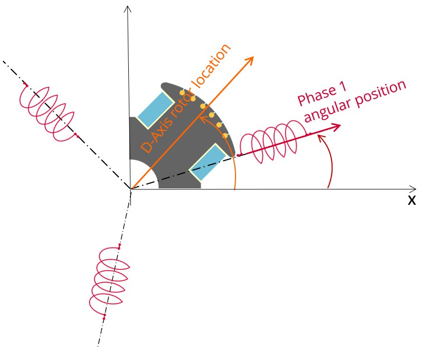
Figure 2. Definition of rotor initial position – Rules for direction

The winding axis of the reference phase is defined from the phase shift of the first electrical harmonic of the magneto motive force (M.M.F.).

Mesh order

To get the results, Finite Element Modelling computations are performed.

The geometry of the machine is meshed.

Two levels of meshing can be considered: First order and second order.

This parameter influences the accuracy of results and the computation time.

By default, second order mesh is used.

Airgap mesh coefficient

The advanced user input “Airgap mesh coefficient” is a coefficient which adjusts the size of mesh elements inside the airgap. When the value of “Airgap mesh coefficient” decreases, the mesh elements get smaller, leading to a higher mesh density inside the airgap, increasing the computation accuracy.

The imposed Mesh Point (size of mesh elements touching points of the geometry), inside the Altair Flux software, is described as:

MeshPoint = (airgap) x (airgap mesh coefficient)

Airgap mesh coefficient is set to 1.5 by default.

The variation range of values for this parameter is [0.05; 2].

0.05 giving a very high mesh density and 2 giving a very coarse mesh density.

CAUTION: Be aware, a very high mesh density does not always mean a better result quality. However, this always leads to a huge number of nodes in the corresponding finite element model. So, it means a need for huge numerical memory and increases the computation time considerably.

The impact of the airgap mesh coefficient on resultant meshing is illustrated bellow: