Inputs

Standard inputs ––––--

Current definition mode

There are 2 common ways to define the electrical current.

Electrical current can be defined by the current density in electric conductors.

In this case, the current definition mode should be « Density ».

Electrical current can be defined directly by indicating the value of the line current (the RMS value is required).

In this case, the current definition mode should be « Current ».

Max. field current density

When the choice of field current definition mode is “Density”, the maximum DC value of the current density in electric conductors “Max. field current density” (Maximum current density) must be provided.

Note: The number of parallel paths is automatically considered in the results.

Max. field current

When the choice of field current definition mode is “Current”, the maximum DC value of the field current supplied to the machine “Max. field current” (Maximum field current) must be provided.

Note: The number of parallel paths is automatically considered in the results.

Speed

Operating speed of the machine to be used in the successive back-EMF tests performed to build the No-load characteristics curve.

Note: Once the computation is performed, it is possible to change the speed and update the results instantaneously.

Back emf target point

The main principle of the No-load test is to perform successive Back EMF tests for different values of field current, to extract a Back-EMF versus the field current curve. However, the full results of those Back EMF tests are not displayed.

This input allows the user to indicate if a full Back-EMF test, and its results, should be presented in the output section. The default option is “No”.

Field current

When the choice of current definition mode is “Current”, the DC value of the current supplied to the field winding: “Field current” (Current in Field conductors) must be provided.

Field current density

When the choice of current definition mode is “Density”, the DC value of the current density in electric conductors “Field current density” (Current density in Field conductors) must be provided.

Note: The number of parallel paths is automatically considered in the results.

Advanced inputs ––––--

No. comp. for if

Computation of the back-EMF:
To compute the Back-EMF for different magnetization states, the field current If is discretized from zero to its maximum value.
The number of computation points for the If discretization can be defined with the user input « No. comp. for If » (Number of computations for field current).
The default value is equal to 6. This default value provides a good compromise between the accuracy of results and computation time. The minimum allowed value is 5.
Computation of maps in Jd,Jq plan:
To get maps along the If dimension, the field current is discretized from zero to its maximum value. The number of computation points along the If - axis can be defined with the user input « No. comp. for If » (Number of computations for If - axis field currents).
The default value is equal to 6. This default value provides a good compromise between the accuracy of results and computation time. The minimum allowed value is 5.
Note: If one uses more than one quadrant, the total number of computations for Jd and Jq will be calculated based on the No. comp. for current Jd, Jq input and the number of quadrants. For example, if No. comp. for current Jd, Jq is set to 10 and the quadrant is set to “1st and 2nd “, then the total number of computations for Jd is 10, but 19 for Jq considering Jd = 0 is shared between both quadrants

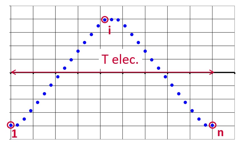
No. comp. / elec. period

The number of computations per electrical period “No. comp. / elec. period” (Number of computations per electrical period) influences the accuracy of results and the computation time.

The default value is equal to 40. The minimum allowed value is 13. This default value provides a good compromise between the accuracy of results and computation time.

Note: The real number of computations per electrical period can be equal to the requested one +/- 1. That is due to our internal computation process since the raw computation is performed over one electrical half period. The result of a whole electrical period is rebuilt from the raw data.

Figure 1. Number of computations per electrical period

Maximum harmonic order

To get the Back-EMF versus time, the flux through each phase of the machine is computed versus rotor angular position.

Harmonics are extracted from the frequency analysis (F.F.T. Fast Fourier Transform) of the Back-EMF signal versus time.

The order of harmonics displayed on bar graphs and in tables can be selected with this advanced user input parameter “Max. harmonic order” (Maximum harmonic order selected for visualization).

Note: From a mathematical point of view, the maximum allowed harmonic order depends on the number of computations per electrical period. In case of a too small number of computations per electrical period, the maximum harmonic order considered will be lower than the one set up by the user.

The default value is equal to 20. The minimum allowed value is 1.

Rotor initial position

By default, the “Rotor initial position” is set to “Auto”.

When the “Rotor initial position mode” is set to “Auto”, the initial position of the rotor is automatically defined by an internal process.

The resulting relative angular position corresponds to the alignment between the axis of the stator phase 1 (reference phase) and the direct axis of the rotor.

When the “Rotor initial position” is set to “User input” (i.e. toggle button on the right), the initial position of the rotor considered for computation must be set by the user in the field « Rotor initial position ». The default value is equal to 0. The range of possible values is [-360, 360].

Notice: The computations are performed by considering the relative angular position between the rotor and stator.

This relative angular position corresponds to the angular distance between the direct axis of the rotor north pole and the axis of the stator phase 1 (reference phase).

The value of the rotor D-axis location, which is automatically defined for each saliency part.

Below is illustrated the Rotor and stator phase relative position

The relative angular position between the axis of the stator phase 1 (reference phase) and the rotor D-axis position must be controlled to perform the tests. See the picture below which will allow defining the working point of the machine.

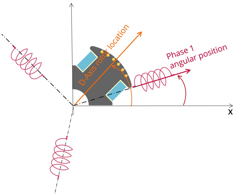
Figure 2. Definition of rotor initial position – Rules for direction

The winding axis of the reference phase is defined from the phase shift of the first electrical harmonic of the magneto motive force (M.M.F.).

Skew model – No. of layers

When the rotor magnets or the stator slots are skewed, the number of layers used in Altair Flux Skew environment to model the machine can be modified: “Skew model - No. of layers” (Number of layers for modelling the skewing in Flux Skew environment).

Note: When there is magnet step skew topology, the number of layers is defined at the design level.

Mesh order

To get the results, Finite Element Modelling computations are performed.

The geometry of the machine is meshed.

Two levels of meshing can be considered: First order and second order.

This parameter influences the accuracy of results and the computation time.

By default, second order mesh is used.

Airgap mesh coefficient

The advanced user input “Airgap mesh coefficient” is a coefficient which adjusts the size of mesh elements inside the airgap. When the value of “Airgap mesh coefficient” decreases, the mesh elements get smaller, leading to a higher mesh density inside the airgap, increasing the computation accuracy.

The imposed Mesh Point (size of mesh elements touching points of the geometry), inside the Altair Flux software, is described as:

MeshPoint = (airgap) x (airgap mesh coefficient)

Airgap mesh coefficient is set to 1.5 by default.

The variation range of values for this parameter is [0.05; 2].

0.05 giving a very high mesh density and 2 giving a very coarse mesh density.

CAUTION: Be aware, a very high mesh density does not always mean a better result quality. However, this always leads to a huge number of nodes in the corresponding finite element model. So, it means a need for huge numerical memory and increases the computation time considerably.

The impact of the airgap mesh coefficient on resultant meshing is illustrated bellow: