Inputs

Standard inputs ––––--

Torque-Speed envelope

Overview

By default, with the “Auto” mode, the list of working points is automatically built by considering seven points on the machine torque-speed envelope. The torque-speed envelope depends on the four following input parameters:

Max. line current, rms
Max. Line-Line voltage, rms
Command mode
Maximum speed

It is also possible to define our own working point list by filling in a table with the targeted speeds and torques.

Table 1. Two ways for defining the working point list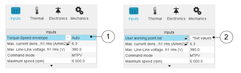

1	Automatic mode: working points are automatically considered on the torque-speed envelope
2	We can define our own working point list by filling in a table with the targeted speeds and torques

Process to define the working point list

Two ways are possible to define the list of working points: either filling the table line per line or by importing an Excel file in which all the working points to be considered are defined.

Table 2. List of working points to be defined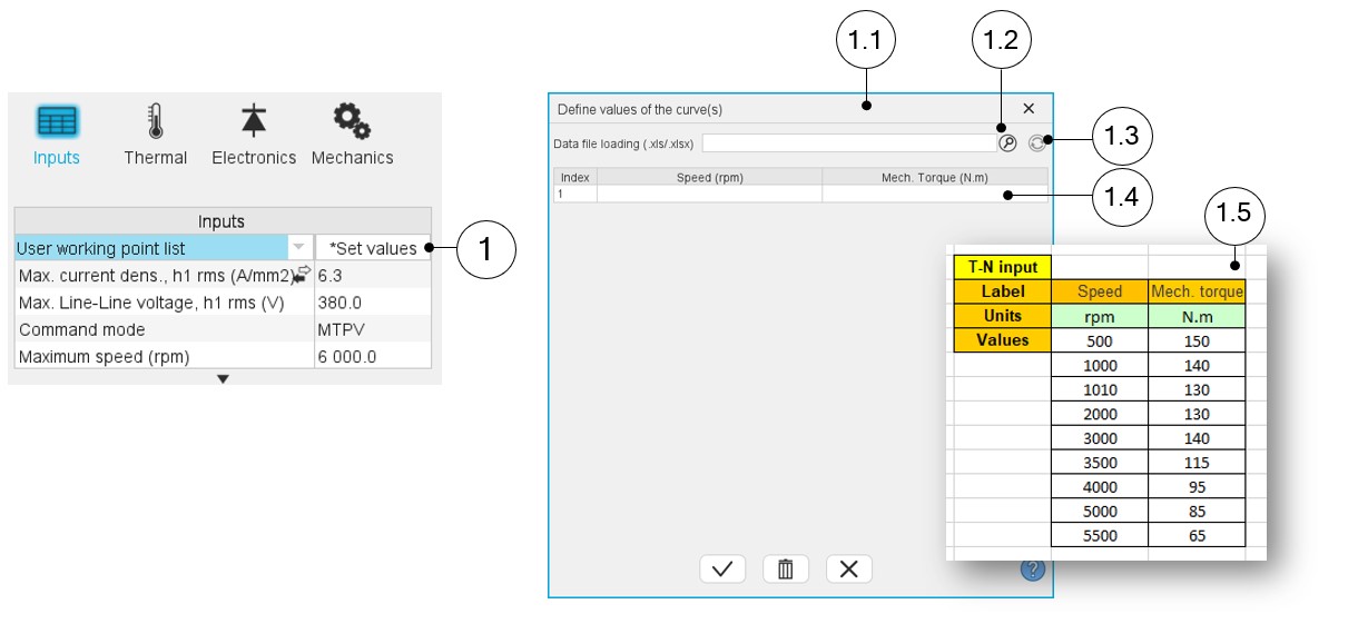

1	Click on the button “Set values” of the field “User working point list” to define the working points in a dialog box.
1.1	Dialog box opened after having clicked on the button “Set values” in the field “Cycle description”.
1.2	Browse the folder to select an Excel file which describes the duty cycle.
1.3	Button to refresh the table data when the considered Excel file has been modified.
1.4	Fields to be filled with data to describe the duty cycle to be considered.
1.5	Excel file template to define the list of working points.

Current definition mode

There are 2 common ways to define the electrical current.

Electrical current can be defined by the current density in electric conductors.

In this case, the current definition mode should be « Density ».

Electrical current can be defined directly by indicating the value of the line current (the RMS value is required).

In this case, the current definition mode should be « Current ».

Max. line current, h1 rms

When the choice of current definition mode is “Current”, the maximum rms value of the line current supplied to the machine “Max. line current, h1 rms” (Maximum line current, first harmonic rms value) must be provided.

Note: The number of parallel paths and the winding connections are automatically considered in the results.

Max. current dens. h1, rms

When the choice of current definition mode is “Density”, the maximum rms value of the current density in electric conductors “Max. current dens., h1 rms” (Maximum current density in conductors, first harmonic rms value) must be provided.

Note: The number of parallel paths and the winding connection are automatically considered in the results.

Max. Line-Line voltage, h1 rms

To supply the machine the rms value of the maximum Line-Line voltage: “Max. Line-Line voltage, h1 rms” (Maximum Line-Line voltage, first harmonic rms value) must be provided.

Note: The number of parallel paths and the winding connection are automatically considered in the results.

Maximum speed

The computation and analysis of the torque-speed curves are performed over a given speed range.

The maximum allowed value for the « Maximum speed » corresponds to 53000 rad/s - about 506000 rpm.

Note: The maximum speed is considered build the following outputs:

Radiated sound power spectrograms versus engine order or frequency
Overall radiated sound power per engine order versus speed
Overall weighted radiated sound power versus speed

Note: As a function of the maximum speed value, following different cases must be considered:

Case 1: The maximum speed is lower than the base speed Nbase (corner point speed of the torque-speed curve) Nmax < Nbase.
In that case, whatever the command mode (MTPA or MTPV), the behavior of the machine will be studied over the speed range [0, Nmax].
That allows the user to precisely choose the range of speed to be considered for computing and displaying the torque-speed curve and especially maps like efficiency maps.
Case 2: The maximum speed is greater than the base speed (corner point speed) Nmax > Nbase.
The relevance of the maximum speed given by the user is analyzed to evaluate if it is reachable by the machine.
If the user maximum speed is unreachable by the machine, the correction of this value is automatically performed.
The resulting new maximum speed is linked to a limit torque. This limit torque is obtained by applying a reduction coefficient to the base point torque.

Note: For additional information on this topic, please see the section dedicated to command modes (Performance mapping – efficiency map)

Advanced inputs ––––--

Max. engine order

Two kinds of inputs are possible: either set an engine order or a number of points per electrical period. Define the Max. engine order (Maximum engine order) or the No. points / elec. period (Number of points per electric period).

When decomposing the Maxwell pressure, applied on the stator, to get its harmonic contributions, the “max. engine order” (Maximum engine order) is required to compute its decomposition in function of the time.

At a practical point of view, when the maximum engine order is equal to N, that leads to consider 2*N computation points over a complete rotation period of the rotor.

Note: The input "Engine order" is in connection with the frequency of vibration.

"Engine order" refers to a mechanical revolution period of the motor whereas frequency refers to the considered electrical period.

Obviously, both are linked with speed.

For instance, radiated sound power can be displayed either by considering frequency or engine order.

No. points / elec. period

The second possibility is to set a “No. points / elec. Period” meaning a number of points per electrical period.

For transient computations the minimum needed number of points per electrical period is 40.

So, when the engine order is not high enough to reach this constraint, It is automatically modified to get 40 computation points per electrical period.

Max. mode / spatial order

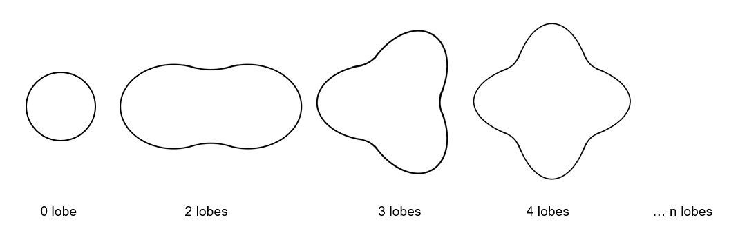
The “max. mode / spatial order” (Maximum mode / spatial order) input allows the user to define the number of modes to be considered for the acoustic structural analysis. If the user selects 25, it means that the highest number of lobes in the stator deformation will be equal to 25 lobes. All deformations corresponding to more than 25 lobes will be dismissed.

Figure 1. Number of lobes of the stator mechanical structure

No. points / tooth pitch

The “No. comp. / tooth pitch” (Number of computations per tooth pitch) allows to choose the number of Maxwell pressure evaluations per tooth. The more points selected, the more accurate the Maxwell pressure harmonic decomposition will be.

No. points for speed interpolation

The “No. points for speed interpolation” (Number of points for speed interpolation) allows to manage the computation of the radiated sound power per engine order. It allows to manage the data interpolation between the speeds indicated as inputs. Thanks to that, the curves “Radiated sound power per engine order versus speed” and “weighted radiated sound power versus speed” can have a better discretization which leads to a better displaying of the local peaks.

The default value is equal to 100. The range of possible values is [50,300]

No. comp. for Jd,Jq

To get maps in the Jd-Jq plan, a grid is defined. The number of computation points along the d-axis and q-axis can be defined with the user input « No. comp. for current Jd, Jq » (Number of computations per quadrant for D-axis and Q-axis phase currents).

The default value is equal to 5. This default value provides a good compromise between the accuracy of results and computation time. The minimum allowed value is 5.

No. comp. for speed

The “No. comp. for speed” (Number of computations for speed) corresponds to the number of points to be considered in the speed range from 0 to the maximum speed.

Half of these points are distributed from 0 to the base speed. The remaining points are distributed from the base speed to the maximum speed.

In both cases, base speed is considered as an additional point.

Note: If the user input parameter “No. comp. for speed” is an odd number, one discretization point is automatically removed.

Figure 2. Definition of the number of computations for speed

The default value is equal to 15, the minimum allowed value is 5. The maximum recommended value is 40.

Note: Increasing the number of computations can improve the convergence of the optimization used to define the torque-speed curve and the efficiency map. However, that also means longer computation time.

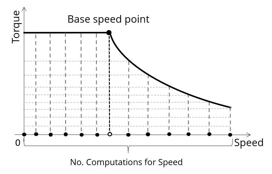
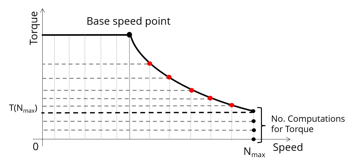
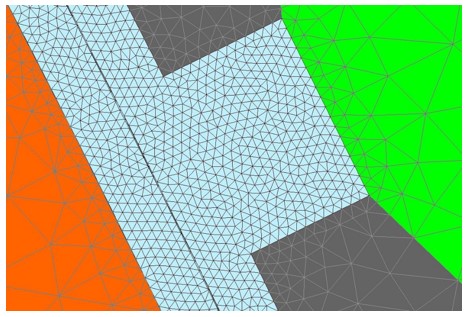
No. comp. for torque

For the speed range [Nbase; Nmax.], the number of computations for torque is imposed by the number of computations for speed in the speed range [Nbase; Nmax.] (Red points in the image shown below).

The advanced user input parameter “No. comp. for torque” allows to finalize the grid within the torque range [0, T (Nmax.)] at the maximum speed (Black points in the image shown below).

The default value is equal to 7. The minimum allowed value is 3. The maximum recommended value is 20.

Figure 3. Definition of the number of computations for torque – MTPV command mode

Mesh order

To get the results, Finite Element Modelling computations are performed.

The geometry of the machine is meshed.

Two levels of meshing can be considered: First order and second order.

This parameter influences the accuracy of results and the computation time.

By default, second order mesh is used.

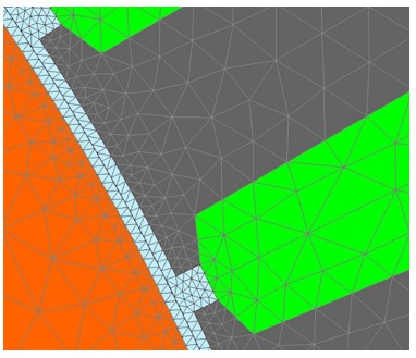
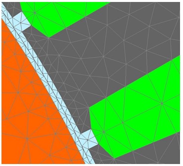
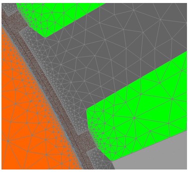
Airgap mesh coefficient

The advanced user input “Airgap mesh coefficient” is a coefficient which adjusts the size of mesh elements inside the airgap. When the value of “Airgap mesh coefficient” decreases, the mesh elements get smaller, leading to a higher mesh density inside the airgap, increasing the computation accuracy.

The imposed Mesh Point (size of mesh elements touching points of the geometry), inside the Altair Flux software, is described as:

MeshPoint = (airgap) x (airgap mesh coefficient)

Airgap mesh coefficient is set to 1.5 by default.

The variation range of values for this parameter is [0.05; 2].

0.05 giving a very high mesh density and 2 giving a very coarse mesh density.

CAUTION: Be aware, a very high mesh density does not always mean a better result quality. However, this always leads to a huge number of nodes in the corresponding finite element model. So, it means a need for huge numerical memory and increases the computation time considerably.

The impact of the airgap mesh coefficient on resultant meshing is illustrated bellow:

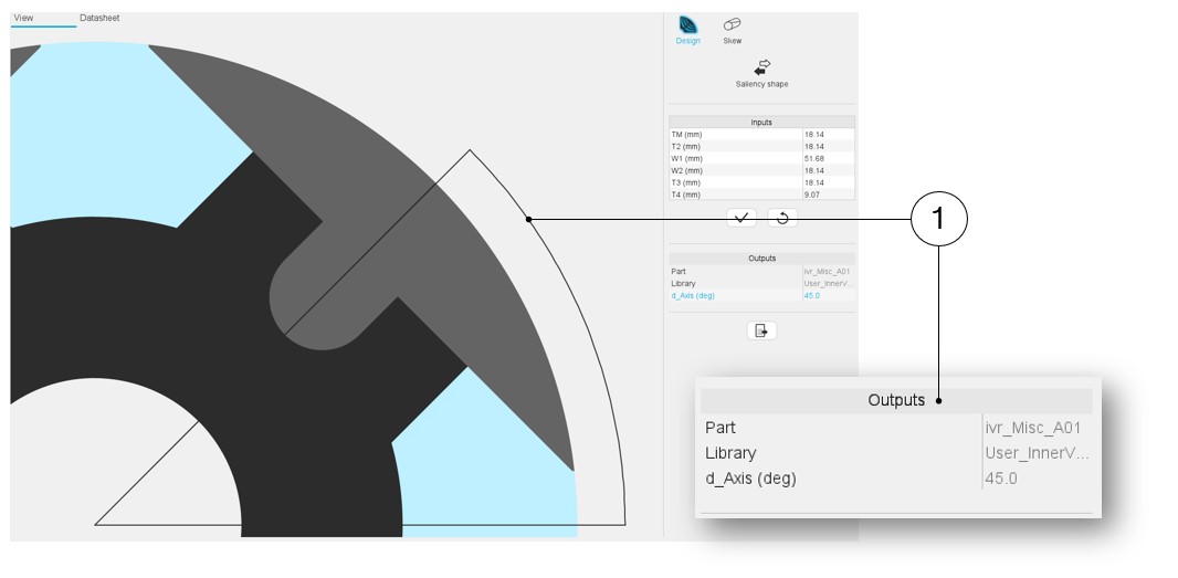
Figure 4. Airgap mesh coefficient = 0.45 = default value

Figure 7. Airgap mesh coefficient = 0.1 (zoomed view)

Rotor d-axis location

The computations are performed by considering a relative angular position between rotor and stator.

For the reluctance synchronous machines, the rotor d-axis location is defined and automatically used to perform computations.

This value is characterized by the saliency topology. This is important to keep in mind this information it.

Rotor initial position

The winding axis of the reference phase is defined from the phase shift of the first electrical harmonic of the magneto motive force (M.M.F.).

The rotor d-axis location is characterized by the saliency topology.

The relative angular position between the axis of the stator phase 1 (reference phase) and the rotor D-axis position must be controlled to perform the tests. See the picture below which will allow defining the working point of the machine.

Here is the representation below of the rotor and stator phase relative position.

The relative angular position between the axis of the stator phase 1 (reference phase) and the rotor D-axis position must be controlled to perform the tests.

The winding axis of the reference phase is defined from the phase shift of the first electrical harmonic of the magneto motive force (M.M.F.).

This allows us to define the working point of the machine.

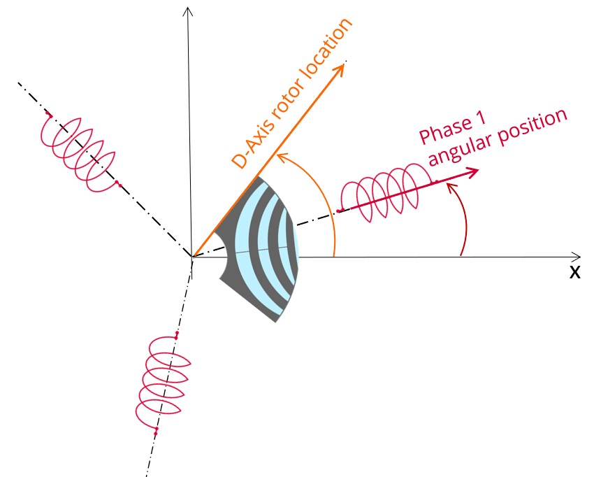
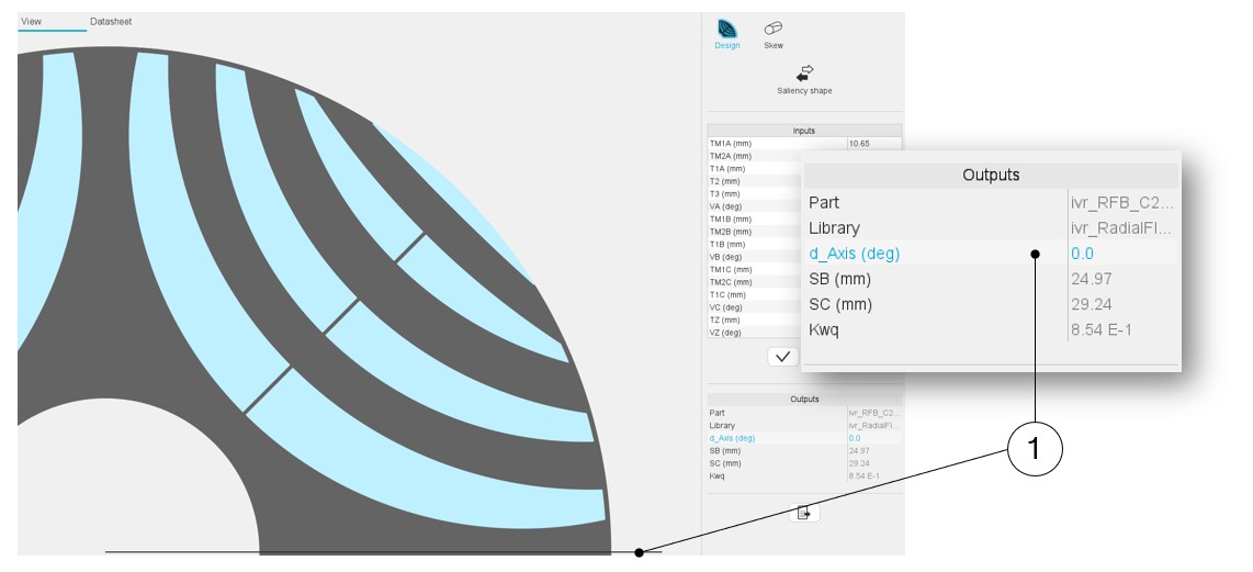
Figure 8. Example of the rotor d-axis location: d-Axis = 0 degree

The rotor d-axis location is an output parameter (read only data) of saliency parts. It completes the description of the topology, and it is automatically used to define the relative position between the axis of the stator phase 1 (reference phase) and the rotor D-axis position for performing the tests when needed.

Figure 9. Example of the rotor d-axis location: d-Axis = 45 degrees (if the rotor yoke, in black, is built with ferromagnetic material)

Advice for use

The modal analysis as well as the radiation efficiency are based on an analytical computation where the stator of the machine is considered as a vibrating cylinder.

The considered cylinder behavior is weighted by the additional masses like the fins or the winding and the subtractive masses like the slots and the cooling circuit holes.

This assumption allows to get fast evaluation of the behavior of machine in connection to NVH. In no way this can replace a mechanical Finite Element modeling and simulation.

Among possible reasons for deviations of results can be the following ones:

The limits of the analytical model are reached or overpassed
Unusual topology and/or dimensions of the teeth/slots
Complexity of the stator-frame structure when it is composed with several components for instance
The ratio between the total length of the frame Lframe and the stack length of the machine Lstk in any case, this ratio must be lower than 1.5: