Inputs

Standard inputs ––––--

Computation modes

There are 2 modes of computation.

The “Fast” computation mode is the default one. It corresponds to a hybrid model which is perfectly suited for the pre-design step. Indeed, all the computations in the back end are based on magnetostatic finite element computations associated to Park transformation. It evaluates the electromagnetic quantities with the best compromise between accuracy and computation time to explore the space of solutions quickly and easily.

The “Accurate” computation mode allows solving the computation with transient magnetic finite element modelling. This mode of computation is perfectly suited to the final design step because it allows getting more accurate results. It also computes additional quantities like the AC losses in winding, rotor iron losses and Joule losses in magnets.

Current definition mode

There are 2 common ways to define the electrical current.

Electrical current can be defined by the current density in electric conductors.

In this case, the current definition mode should be « Density ».

Electrical current can be defined directly by indicating the value of the line current (the RMS value is required).

In this case, the current definition mode should be « Current ».

Line current h1, rms

When the choice of current definition mode is “Current”, the rms value of the line current supplied to the machine: “Line current, h1 rms” (Line current, first harmonic rms value) must be provided.

Current density h1, rms

Control angle

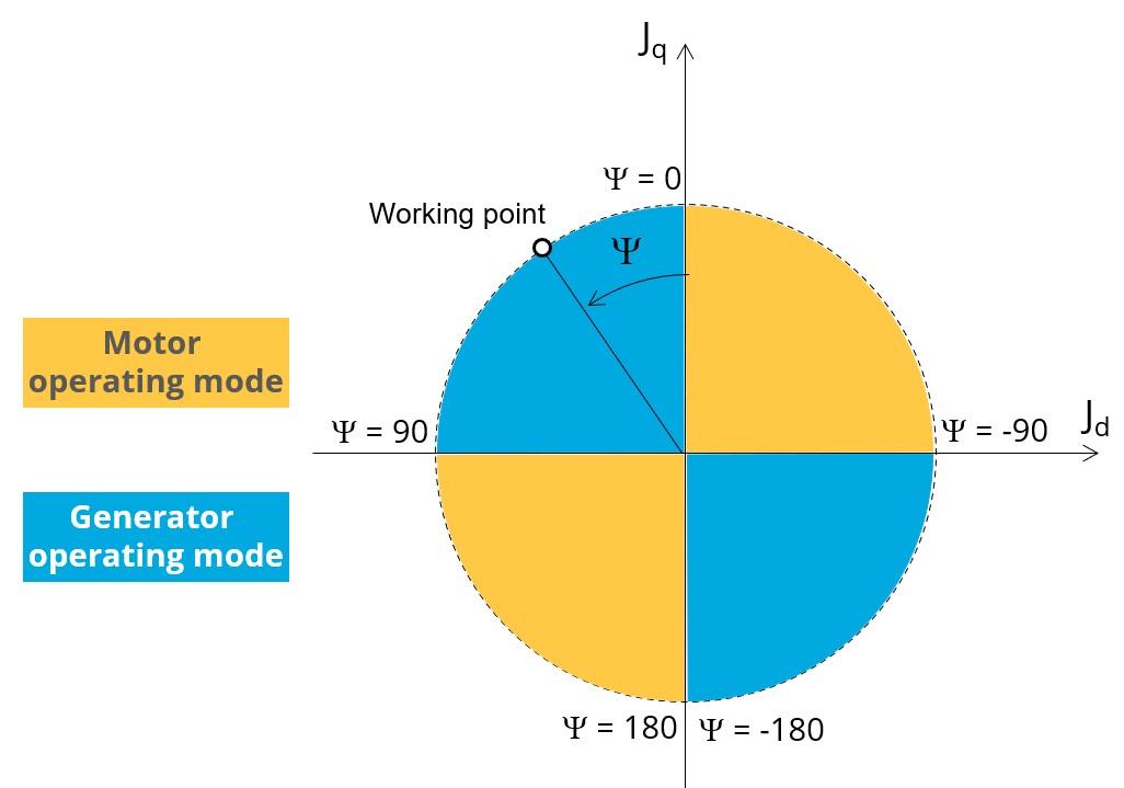
Considering the vector diagram shown below, the “Control angle” is the angle between the Q-axis and the electrical current (J) i.e. (Ψ = (Jq, J)).

The default value is 45 degrees. It is an electrical angle. It must be set in a range of -90 to 90 degrees.

Note: The sign of results like power depends on both the convention and the operating mode.

Speed

The imposed “Speed” (Speed) of the machine must be set.

Rotor position dependency

AC losses analysis - Fast

The “AC losses analysis - Fast” (AC losses analysis required only while “Fast” computation mode and Rotor position dependency are selected) allows computing or not AC losses in stator winding. There are two available options:

None: AC losses are not computed. However, as the computation mode is “Fast” with rotor position dependency, a multi-static computation is performed without representing the solid conductors (wires) inside the slots. Phases are modeled with coil regions. Thus, the mesh density (number of nodes) is lower which leads to a lower computation time.

FE-Hybrid: AC losses in winding are computed without representing the wires (strands, solid conductors) inside the slots.

Since the location of each wire is accurately defined in the winding environment, sensors evaluate the evolution of the flux density close each wire. Then, a postprocessing based on analytical approaches computes the resulting current density inside the conductors and the corresponding Joule losses.

The wire topology can be “Circular” or “Rectangular”.

There can be one or several wires in parallel (in hand) in a conductor (per turn).

AC losses analysis - Accurate

The “AC losses analysis - Accurate” (AC losses analysis required only while “Accurate” computation mode is selected) allows computing or not AC losses in stator winding. There are three available options:

None: AC losses are not computed. However, as the computation mode is “Accurate”, a transient computation is performed without representing the solid conductors (wires) inside the slots. Phases are modeled with coil regions. Thus, the mesh density (number of nodes) is lower which leads to a lower computation time.

FE-One phase: AC losses are computed with only one phase modeled with solid conductors (wires) inside the slots. The other two phases are modeled with coil regions. Thus, AC losses in winding are computed with a lower computation time than if all the phases were modeled with solid conductors. However, this can have a little impact on the accuracy of results because we have supposed that the magnetic field is not impacted by the modeling assumption.

FE-All phase: AC losses are computed, with all phases modeled with solid conductors (wires) inside the slots. This computation method gives the best results in terms of accuracy, but with a higher computation time.

FE-Hybrid: AC losses in winding are computed without representing the wires (strands, solid conductors) inside the slots.

Since the location of each wire is accurately defined in the winding environment, sensors evaluate the evolution of the flux density close each wire. Then, a postprocessing based on analytical approaches computes the resulting current density inside the conductors and the corresponding Joule losses.

The wire topology can be “Circular” or “Rectangular”.

There can be one or several wires in parallel (in hand) in a conductor (per turn).

Advanced inputs ––––--

No. computed elec. periods

The user input “No. computed elec. periods” (Number of computed electrical periods only required with “Accurate” computation mode) influences the accuracy of results especially in case of AC losses computation. Indeed, with represented conductors (AC losses analysis set to “FE - One phase” or “FE - All phase”) the computation may lead to have transient current evolution in wires requiring more than an electrical period of simulation to reach the steady state over an electrical period.

The default value is equal to 2. The minimum allowed value is 0.5 (recommended with AC losses analysis set to “None”). The default value provides a good compromise between the accuracy of results and computation time.

No. comp. / elec. period

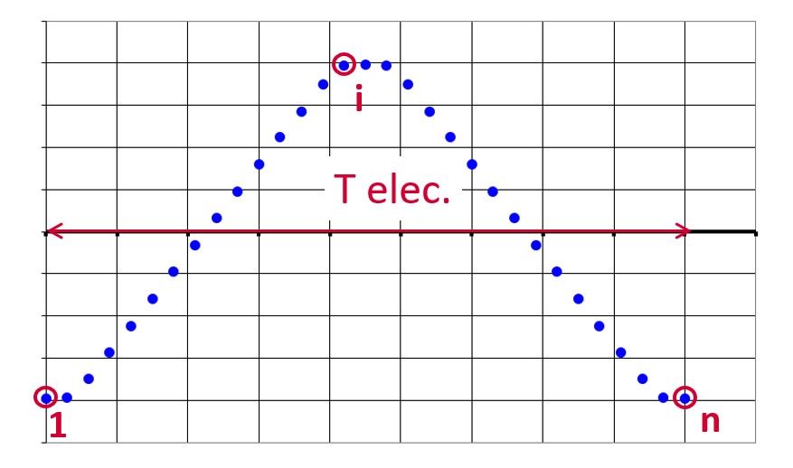
In general, the user input “No. comp. / elec. period” (Number of computed electrical periods) only required with rotor position dependency set to “Yes” influences the accuracy of results (computation of the peak-peak ripple torque, iron losses…) and the computation time.

Skew model – No. of layers

Mesh order

To get the results, Finite Element Modelling computations are performed.

The geometry of the machine is meshed.

Two levels of meshing can be considered: First order and second order.

This parameter influences the accuracy of results and the computation time.

By default, second order mesh is used.

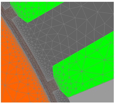
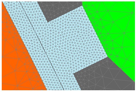
Airgap mesh coefficient

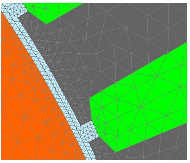
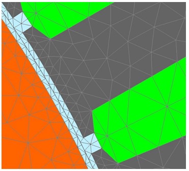
The advanced user input “Airgap mesh coefficient” is a coefficient which adjusts the size of mesh elements inside the airgap. When the value of “Airgap mesh coefficient” decreases, the mesh elements get smaller, leading to a higher mesh density inside the airgap, increasing the computation accuracy.

The imposed Mesh Point (size of mesh elements touching points of the geometry), inside the Altair Flux software, is described as:

MeshPoint = (airgap) x (airgap mesh coefficient)

Airgap mesh coefficient is set to 1.5 by default.

The variation range of values for this parameter is [0.05; 2].

Convergence criteria on temperature

The advanced user input “Converg. Criteria on temperature” (Convergence criteria on temperature) is a percentage driving the convergence of the computation.

This advanced user input is available when the iterative thermal solving mode is selected in the thermal settings.

The iterative process (loop between electromagnetic and thermal computations) must run until the convergence criterion has been reached leading to the electromagnetic-thermal steady state. The convergence process is completed when the variation of temperature between two iterations gets lower than the ratio “Converg. Criteria on temperature” set in input.

Convergence criterion on temperature is set to 1.0 % by default.

The variation range of values for this percentage is ]0;10].

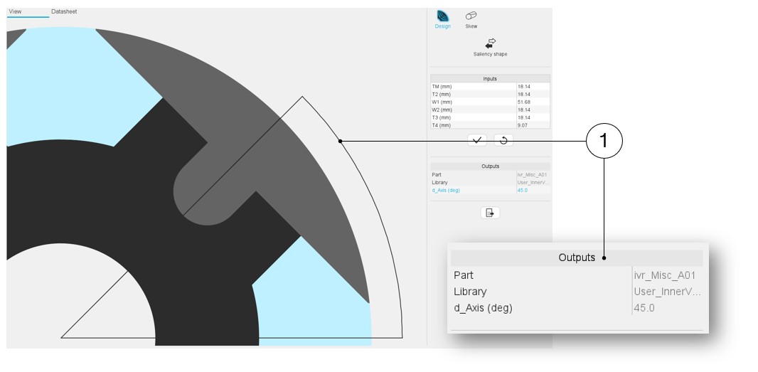
Rotor d-axis location

The computations are performed by considering a relative angular position between rotor and stator.

For the reluctance synchronous machines, the rotor d-axis location is defined and automatically used to perform computations.

This value is characterized by the saliency topology. This is an important information to keep in mind.

For additional information please refer to the section Rotor initial position.

Rotor initial position

The winding axis of the reference phase is defined from the phase shift of the first electrical harmonic of the magneto motive force (M.M.F.).

The rotor d-axis location is characterized by the saliency topology.

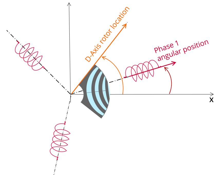
The relative angular position between the axis of the stator phase 1 (reference phase) and the rotor D-axis position must be controlled to perform the tests. See the picture below which will allow defining the working point of the machine.

Here is the representation below of the rotor and stator phase relative position.

The relative angular position between the axis of the stator phase 1 (reference phase) and the rotor D-axis position must be controlled to perform the tests.

The winding axis of the reference phase is defined from the phase shift of the first electrical harmonic of the magneto motive force (M.M.F.).

This allows us to define the working point of the machine.

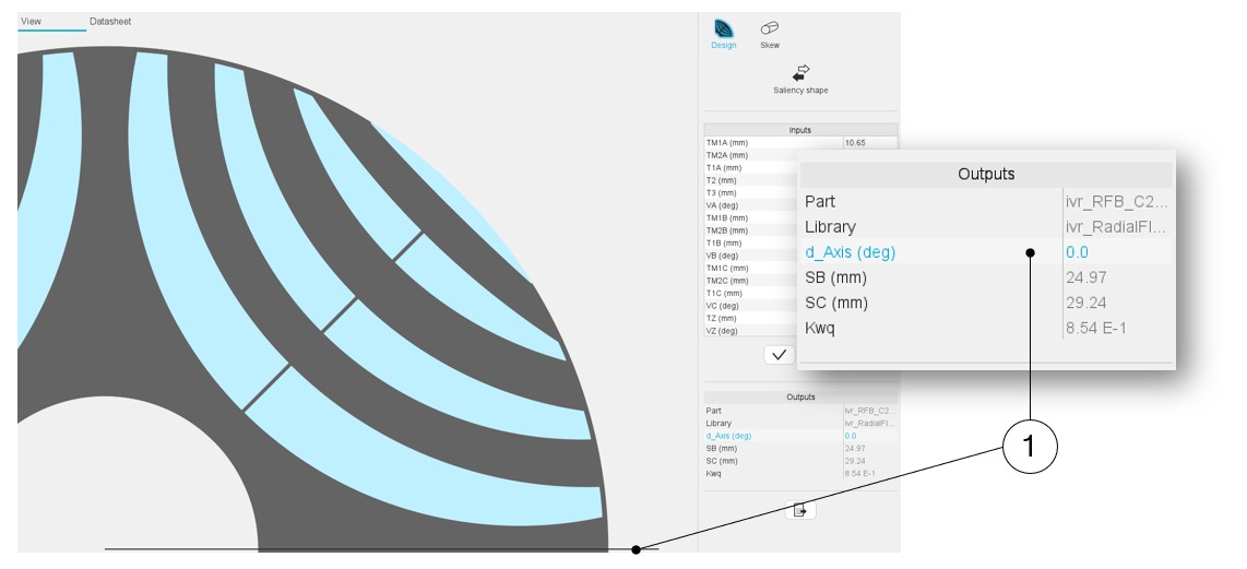
The rotor d-axis location is an output parameter (read only data) of saliency parts. It completes the description of the topology, and it is automatically used to define the relative position between the axis of the stator phase 1 (reference phase) and the rotor D-axis position for performing the tests when needed.

Advice for use