Inputs

Standard inputs ––––--

Current definition mode

There are 2 common ways to define the electrical current.

Electrical current can be defined by the current density in electric conductors.

In this case, the current definition mode should be « Density ».

Electrical current can be defined directly by indicating the value of the line current (the RMS value is required).

In this case, the current definition mode should be « Current ».

Max. line current, h1 rms

When the choice of current definition mode is “Current”, the maximum rms value of the line current supplied to the machine “Max. line current, h1 rms” (Maximum line current, first harmonic rms value) must be provided.

Note: The number of parallel paths and the winding connections are automatically considered in the results.

Max. current dens. h1, rms

When the choice of current definition mode is “Density”, the maximum rms value of the current density in electric conductors “Max. current dens., h1 rms” (Maximum current density in conductors, first harmonic rms value) must be provided.

Note: The number of parallel paths and the winding connection are automatically considered in the results.

Command mode

Two commands are available: Maximum Torque Per Voltage (MTPV) and Maximum Torque Per Amps (MTPA) command mode.

For the base speed point computation, both commands lead to the same results. In fact, the base speed point corresponds to the working point which maximize the mechanical torque at maximum current and at maximum voltage. Following this, MTPA and MTPV commands give the same results on this test.

Note: The computed maximum speed depends on the chosen command mode.

Ripple torque analysis

The “Ripple torque analysis” (Additional analysis on ripple torque period: Yes / No) allows to compute or not to compute the value of the ripple torque and to display the corresponding torque versus the angular position over the corresponding ripple torque period.

The default value is “No”.

Note:

This choice influences the accuracy of results and on the computation time. The peak-peak ripple torque is calculated. This additional computation needs addition computation time.
In case of “Yes”, the ripple torque is computed. Then, the flux density in regions and the magnet demagnetization rate are evaluated through the ripple torque computation.
In case of “No”, the ripple torque is not computed. Then, the flux density in regions and the magnet demagnetization rate are evaluated by considering the Park’s model computation.

Advanced inputs ––––--

No. comp. for ctrl. angle

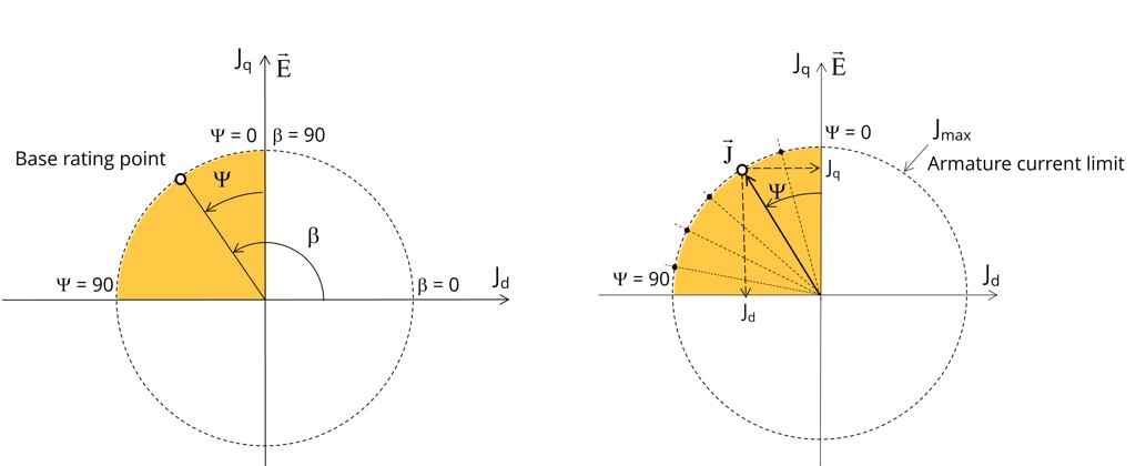
Considering the vector diagram shown below, the control angle Ψ is the angle between the electromotive force E and the electrical current (J) (Ψ = (E, J)).

The computation to get the corner point location is performed by considering control angle (Ψ) over a range of 0 to 90 electrical degrees. The user input “No. comp. for ctrl. angle” (Number of computations for the control angle) allows to choose between accuracy of results and computation time by using a number of computations between and . The variation area for is represented by the quarter circle (colored yellow in the diagram). This discretization is necessary to find the working point corresponding to the base speed point of the torque-speed curve.

The default value of Number of computations for the control angle is equal to 5. The minimum allowed value is 5.

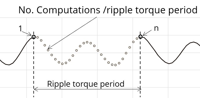
Figure 1. Variation area for control angle Ψ

No. comp. / ripple period

The number of computations per ripple torque period is considered to perform a “Ripple torque analysis”.

The user input “No. comp. / ripple period” (Number of computations per ripple torque period) influences the accuracy of results (computation of the peak-peak ripple torque) and the computation time.

The default value is equal to 30. The minimum allowed value is 25. The default value provides a good compromise between the accuracy of results and computation time.

Figure 2. Definition of the number of computations per ripple torque period

Rotor initial position

By default, the “Rotor initial position” is set to “Auto”

(except in the test Characterization / Cogging where it is a user input whose default value is 0).

When the “Rotor initial position mode” is set to “Auto”, the initial position of the rotor is automatically defined by an internal process of FluxMotor.

The resulting relative angular position corresponds to the alignment between the axis of the stator phase 1 (reference phase) and the direct axis of the rotor north pole.

When the “Rotor initial position” is set to “User input” (i.e. toggle button on the right), the initial position of the rotor considered for computation must be set by the user in the field « Rotor initial position ». The default value is equal to 0. The range of possible values is [-360, 360].

Notice: The relative angular position between the axis of the stator phase 1 (reference phase) and the direct axis of the rotor north pole must be controlled to perform the tests. See the picture below. That allows defining the working point of the machine.

Figure 3. Definition of rotor initial position – Rules for direction

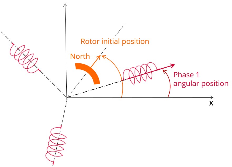
The winding axis of the reference phase is defined from the phase shift of the first electrical harmonic of the magneto motive force (M.M.F.).

By convention, a field pole "North” corresponds to a magnetic flux density vector oriented towards exterior of the rotor.

Note: In the test Characterization / Cogging there is a user input whose default value is 0, no Auto mode available.

Skew model – No. of layers

When the rotor magnets or the stator slots are skewed, the number of layers used in Altair Flux Skew environment to model the machine can be modified: “Skew model - No. of layers” (Number of layers for modelling the skewing in Flux Skew environment).

Note: When there is magnet step skew topology, the number of layers is defined at the design level.

Mesh order

To get the results, Finite Element Modelling computations are performed.

The geometry of the machine is meshed.

Two levels of meshing can be considered: First order and second order.

This parameter influences the accuracy of results and the computation time.

By default, second order mesh is used.

Airgap mesh coefficient

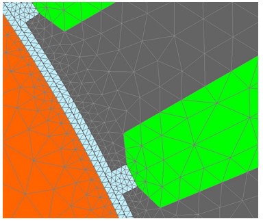
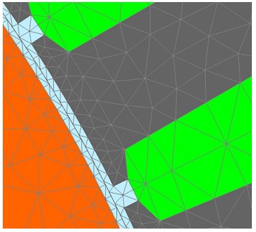
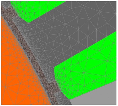
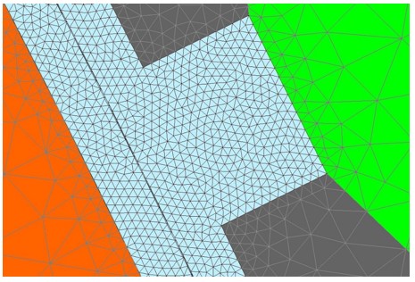
The advanced user input “Airgap mesh coefficient” is a coefficient which adjusts the size of mesh elements inside the airgap. When the value of “Airgap mesh coefficient” decreases, the mesh elements get smaller, leading to a higher mesh density inside the airgap, increasing the computation accuracy.

The imposed Mesh Point (size of mesh elements touching points of the geometry), inside the Altair Flux software, is described as:

MeshPoint = (airgap) x (airgap mesh coefficient)

Airgap mesh coefficient is set to 1.5 by default.

The variation range of values for this parameter is [0.05; 2].

0.05 giving a very high mesh density and 2 giving a very coarse mesh density.

CAUTION: Be aware, a very high mesh density does not always mean a better result quality. However, this always leads to a huge number of nodes in the corresponding finite element model. So, it means a need for huge numerical memory and increases the computation time considerably.

The impact of the airgap mesh coefficient on resultant meshing is illustrated bellow:

Figure 4. Airgap mesh coefficient = 0.45 = default value

Figure 7. Airgap mesh coefficient = 0.1 (zoomed view)