lsim
Simulates LTI model response to arbitrary inputs.
Syntax
[Y, T, X] = lsim(SYS, U)
[Y, T, X] = lsim(SYS, U, T)
[Y, T, X] = lsim(SYS, U, T, X0)
Inputs
- SYS
- A state-space or transfer function model. The model must have at least as many poles as zeros.
- U
- The signal vector.
- T
- The time vector.
- X0
- The state vector initial conditions. Default = a zero vector.
Outputs
- Y
- The output response matrix.Note: The outputs are stored by column.
- T
- The time vector.
- X
- The state trajectories matrix. Note: The trajectories are stored by column.
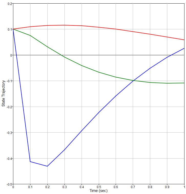
Example
Plot state trajectories:
Figure 1.
Figure 1.
 A = [-20 -40 -60;1  0  0; 0  1  0];
B = [1;   0;   0];
C = [0   0   1];
D = 0;
T = [0:0.1:1];        % Time vector
U = zeros(size(T,1), size(T,2));
X0 = [0.1 0.1 0.1];   % Initial Condition
sys = ss(A, B, C, D);
[y, t, x] = lsim(sys, U, T, X0);
plot(t,x);
xlabel('Time (sec)');
ylabel('State Trajectory');
grid;