Learn how to simulate and review results for the model
SineIntegral.scm.
Files for This Tutorial
SineIntegral.scm
A finished version of the models you build in the tutorials along with any files
required to complete the tutorials are available at this location:
<installation_directory>/tutorial_models/.
Setting Block Parameters
Set parameters for the SineWaveGenerator block.
Load the model SineIntegral_practice.scm that you created
in the tutorial, Tutorial: Creating a Simple Block Diagram, or from the tree in
the Demo Browser, select
tutorial_models/SineIntegral.scm
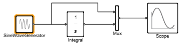
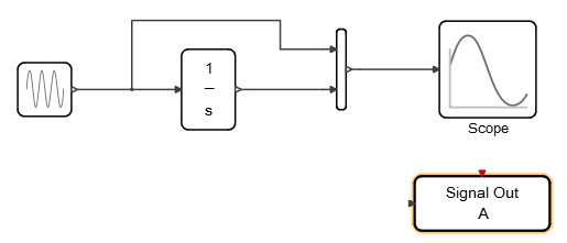
On the SineWaveGenerator block, shown highlighted in the
following figure, double-click, or right-click, and from the context menu,
select Parameters.
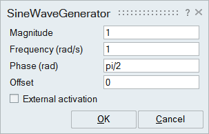
For the parameter Phase(rad), enter pi/2, and then click
OK.
The value you enter shifts the sine wave by a quarter period to obtain a
cosine wave.
Setting Simulation Parameters
Define the simulation time parameters for the analysis.
On the ribbon, select the Setup tool.
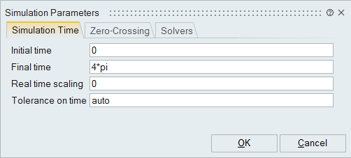
On the Simulation Parameters dialog that appears, select
the Simulation Time tab.
For the parameter, Final Time, enter
4*pi, which is twice the value of a sine wave
period.
Select the Solvers tab.
From the Select a Solver pull down menu, select: LSODA,
and then select OK.
The LSODA solver is an efficient variable-step, variable-order ODE
solver that is suitable for both stiff and non-stiff problems.
Simulating a Model and Plotting Data
Run and review the progress of a simulation with Scope plots.
On the ribbon, from the Simulate tool group, click
Run.
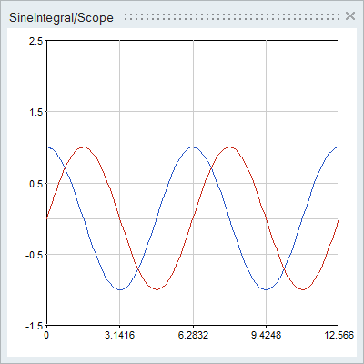
The simulation finishes very quickly, and a Scope window appears with a
plot of the simulation results. If you do not see a Scope window, double-click
the Scope block in the diagram to display the window.
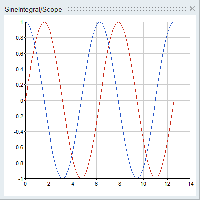
The upper and lower limits of the Y-axis go far beyond the range of a unity
magnitude sine wave. To fit the Scope window to the plot data, middle-mouse
click.
In the tree of the Project Browser, under Scopes & Plots,
double-click SineIntegral/Scope; or right-click
SineIntegral/Scope, and from the context menu, select
Show.
The Scope window appears.
To close the Scope window, right-click, and then select
Close.
Experiment with opening the window again. In the tree of the Project Browser, under Scopes & Plots, double-click
SineIntegral/Scope; or right-click
SineIntegral/Scope, and from the context menu, select
Show.
The Scope window appears.
Right-click, and then select Close.
Exporting a Signal to an OML Workspace
Manipulate data exported to the OML
workspace.
In the diagram, replace the Scope block with a SignalOut block: from the
Palette Browser, double-click the folders Activate > SignalExporters.
Select, and then drag and drop a SignalOut block next to
the diagram, but do not link it to the diagram.
Select the SignalOut block, and then press
Ctrl+
X.
Select the Scope block, and then press
Ctrl+V.
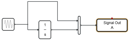
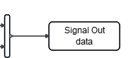
The Scope block is cleared and replaced with the SignalOut block:
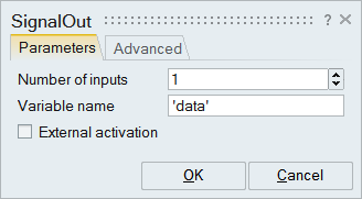
Double-click the SignalOut block.
The block dialog opens to the Parameters
tab.
As you see in the following figure, for Number of inputs, keep the default
value of 1; for Variable name, enter
'data'; if selected, clear the External Activation
check box.
Click OK.
The SignalOut block is updated in the diagram. The new variable name
appears, and the red activation port at the top of block is removed. The block
now inherits activation. If an incoming signal is present, the SignalOut block
is activated.
From the ribbon, select Run.
The simulation results are written to a variable named
“data” in the OML Command
Window. If the OML Command Window is not open by
default, from the menu bar, select View > OML Command Window. The variable is also listed in the Variable Browser. If you do
not see the Variable Browser, from the menu bar, select View > Variable Browser.
In the OML Command Window, enter the following
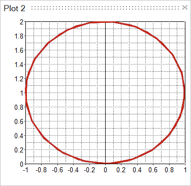
command to plot a curve for the data in row x in respect to row
y:
x = data.ch{1}.data(1,:);
y = data.ch{1}.data(2,:);
plot(x,y);
The
following plot appears:
Press Ctrl+S. In the Save Model
As dialog that appears, for File name,
enter SineIntegralSignalOut_practice.


 .
The simulation results are written to a variable named
.
The simulation results are written to a variable named