Learn how to model and simulate a simple hybrid system that includes discrete signals
and continuous linear systems.
Files for This Tutorial
HybridSystem.scm
A finished version of the models you build in the tutorials along with any files
required to complete the tutorials are available at this location:
<installation_directory>/tutorial_models/.
Overview
The model in this tutorial includes DiscreteDelay blocks to generate a square-wave
signal that is fed into the input of a continuous-time linear system. The continuous-time
linear system is represented by its transfer function via a ContTransFunc block. A Scope
block plots the output of the system.
Constant-coefficient linear differential equations can be expressed in Laplace
domain by applying the Laplace transform to both sides of the equation. This operation
transforms the differential equation into an algebraic equation since the
differentiation operation is converted to multiplication by the independent variable,
s. If the differential equation represents the input-output
behavior of a system in the time domain, the resulting equation in the Laplace domain
can be used to obtain the system’s transfer functions. For example, the linear
differential equation:
yields the transfer function:
The ContTransFunc block can represent a system’s
single-input, single- or possible multi-output, transfer function. The block parameters
contain the coefficients of the transfer function’s denominator and numerator(s). A
special case of the transfer function is an integrator, such as
represented by the Integral block. In discrete-time,
transfer functions are obtained by applying the Z transform to difference equations. The
special case of a unit delay operator is represented by the
DiscreteDelay block. This block is usually activated
periodically by a SampleClock block, which fixes the period and
phase of the activations. Discrete-time signals are updated at activation times and
remain constant from one activation to the next.
Constructing a Discrete Signal
Construct discrete signals with the DiscreteDelay block.
From the ribbon, click or,
from the menu bar, click File > New.
Save your model as HybridSystem_practice.scm.
From the Palette Browser, drag and drop the following
blocks into your diagram:
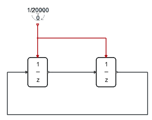
From Activate > Dynamical, drag and drop two DiscreteDelay
blocks into your diagram.
From Activate > ActiveOperations, drag and drop one SampleClock
block into your diagram.
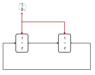
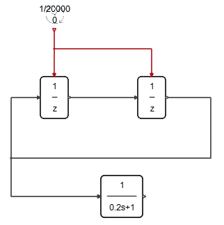
Assemble and connect the blocks in your diagram as you see in the following
figure:
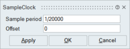
On the SampleClock block, double-click. In the block
dialog, for the Sample period, enter: 1/20000, and click
OK.
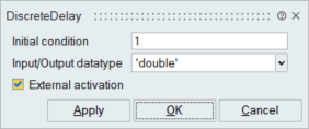
On the block, DiscreteDelay, double-click. In the block
dialog, for Initial Condition, enter: 1, and click
OK.
The discrete signal is constructed as you see in the following figure. The
signal generates a square wave signal toggled between 0 and 1 at the
frequency of 10000Hz.
Creating a Continuous Transfer Function
Represent continuous linear systems with the ContTransFunc block.
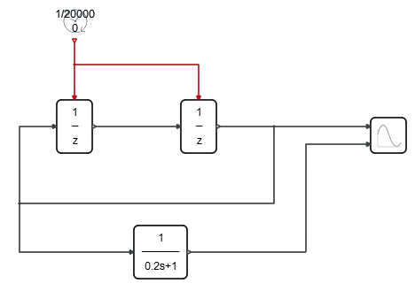
In the Palette Browser, double-click Activate > Dynamical, and drag and drop a ContTransFunc block
into the diagram.
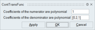
On the block, ContTransFunc, double-click. In the block
dialog, for Coefficients of the numerator polynomial,
enter: 1. For Coefficients of the denominator
polynomial, enter: [0.2 1], and click
OK.
The ContTransFunc block represents a first order linear system that models
the behavior of a simplified motor dynamics.
Connect the block to your diagram as you see in the following figure:
In the Palette Browser, double-click Activate > SignalViewers, and drag and drop one Scope block into
the diagram.
On the Scope block, double-click. For Number of inputs,
enter: 2.
Two input ports appear on the Scope block.
Connect the Scope block to the diagram as you see in the following
figure:
Simulating the Hybrid Model
Set simulation parameters and run a simulation.
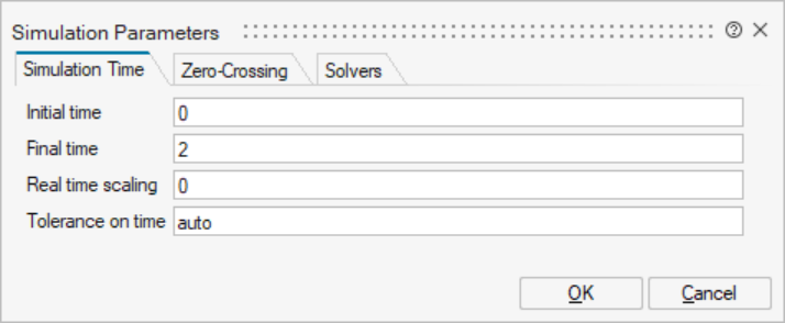
On the ribbon, select the Setup tool.
On the Simulation Parameters dialog, enter 2 for Final
time, then click OK.
On the ribbon, click Run
.
The simulation of the diagram begins.
Reviewing Simulation Data
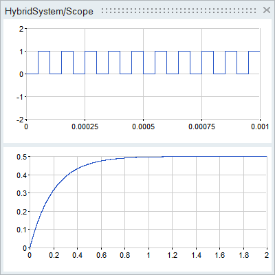
Examine the data in the plots generated from the Scope block.
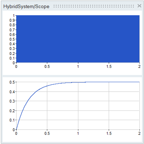
On the Scope block, double-click.
A Scope window opens. Because the Scope block is defined with two
inputs, two corresponding subplots are displayed, representing the square wave
signal and system response, respectively. Because the frequency of the square
wave is 10,000Hz, too many periods exist in the time span between 0 and 2
seconds, therefore zooming into a smaller range is required.
To reveal the square wave form more clearly, on the X-axis of the upper
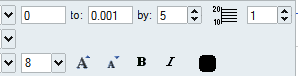
subplot, right-click to launch a floating panel.
For the upper limit value, enter 0.001.
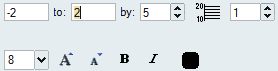
On the Y-axis of the upper subplot, right-click. In the floating panel, for the
lower-limit value, enter: -2; for the upper limit value,
enter: 2.
To fit the view of the plot in the window, on the lower subplot,
middle-click.
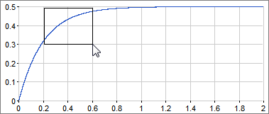
To zoom in on an area in the plot, press the Ctrl key + middle-click + drag to select a
frame on the plot.
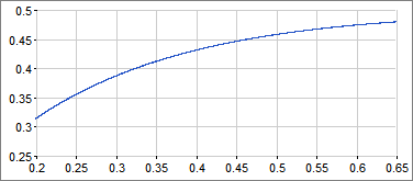
The area in the frame appears in the lower plot as you see in the following
image:
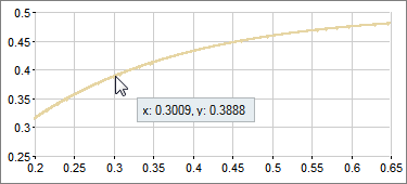
To reveal specific data points on the curve, press and hold the
Ctrl key while
positioning your cursor on the curve.
The data points closest to the cursor are displayed.
 or,
from the menu bar, click .
or,
from the menu bar, click .


 The area in the frame appears in the lower plot as you see in the following image: