 Package Modelica.Blocks.Nonlinear
Library of discontinuous or non-differentiable algebraic control blocks
Package Modelica.Blocks.Nonlinear
This package contains discontinuous and non-differentiable, algebraic input/output blocks.
Extends from Modelica.Icons.Package (Icon for standard packages).
| Name | Description |
|---|---|
DeadZone | Provide a region of zero output |
FixedDelay | Delay block with fixed DelayTime |
Limiter | Limit the range of a signal |
PadeDelay | Pade approximation of delay block with fixed delayTime (use balance=true; this is not the default to be backwards compatible) |
SlewRateLimiter | Limits the slew rate of a signal |
VariableDelay | Delay block with variable DelayTime |
VariableLimiter | Limit the range of a signal with variable limits |
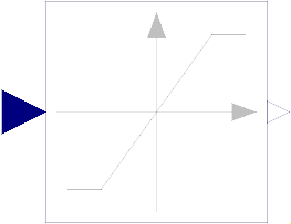 Block Modelica.Blocks.Nonlinear.Limiter
The Limiter block passes its input signal as output signal as long as the input is within the specified upper and lower limits. If this is not the case, the corresponding limits are passed as output.
The parameter homotopyType in the Advanced tab specifies the
simplified behaviour if homotopy-based initialization is used:
NoHomotopy: the actual expression with limits is usedLinear: a linear behaviour y = u is assumed (default option)UpperLimit: it is assumed that the output is stuck at the upper limit u = uMaxLowerLimit: it is assumed that the output is stuck at the lower limit u = uMinIf it is known a priori in which region the input signal will be located, this option can help a lot by removing one strong nonlinearity from the initialization problem.
Extends from Modelica.Blocks.Interfaces.SISO (Single Input Single Output continuous control block).
| Type | Name | Default | Description |
|---|---|---|---|
Real | uMax | Upper limits of input signals | |
Real | uMin | -uMax | Lower limits of input signals |
Boolean | strict | false | = true, if strict limits with noEvent(..) |
LimiterHomotopy | homotopyType | Modelica.Blocks.Types.LimiterHomotopy.Linear | Simplified model for homotopy-based initialization |
Boolean | limitsAtInit | true | Has no longer an effect and is only kept for backwards compatibility (the implementation uses now the homotopy operator) |
| Type | Name | Description |
|---|---|---|
input RealInput | u | Connector of Real input signal |
output RealOutput | y | Connector of Real output signal |
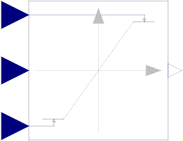 Block Modelica.Blocks.Nonlinear.VariableLimiter
The Limiter block passes its input signal as output signal as long as the input is within the upper and lower limits specified by the two additional inputs limit1 and limit2. If this is not the case, the corresponding limit is passed as output.
The parameter homotopyType in the Advanced tab specifies the
simplified behaviour if homotopy-based initialization is used:
NoHomotopy: the actual expression with limits is usedLinear: a linear behaviour y = u is assumed (default option)Fixed: it is assumed that the output is fixed at the value ySimplifiedIf it is known a priori in which region the input signal will be located, this option can help a lot by removing one strong nonlinearity from the initialization problem.
Extends from Modelica.Blocks.Interfaces.SISO (Single Input Single Output continuous control block).
| Type | Name | Default | Description |
|---|---|---|---|
Boolean | strict | false | = true, if strict limits with noEvent(..) |
VariableLimiterHomotopy | homotopyType | Modelica.Blocks.Types.VariableLimiterHomotopy.Linear | Simplified model for homotopy-based initialization |
Real | ySimplified | 0 | Fixed value of output in simplified model |
Boolean | limitsAtInit | true | Has no longer an effect and is only kept for backwards compatibility (the implementation uses now the homotopy operator) |
| Type | Name | Description |
|---|---|---|
input RealInput | u | Connector of Real input signal |
output RealOutput | y | Connector of Real output signal |
input RealInput | limit1 | Connector of Real input signal used as maximum of input u |
input RealInput | limit2 | Connector of Real input signal used as minimum of input u |
 Block Modelica.Blocks.Nonlinear.SlewRateLimiter
The SlewRateLimiter block limits the slew rate of its input signal in the range of [Falling, Rising].
To ensure this for arbitrary inputs and in order to produce a differential output, the input is numerically differentiated
with derivative time constant Td. Smaller time constant Td means nearer ideal derivative.
Note: The user has to choose the derivative time constant according to the nature of the input signal.
Extends from Modelica.Blocks.Interfaces.SISO (Single Input Single Output continuous control block).
| Type | Name | Default | Description |
|---|---|---|---|
Real | Rising | 1 | Maximum rising slew rate [+small..+inf) [1/s] |
Real | Falling | -Rising | Maximum falling slew rate (-inf..-small] [1/s] |
Time | Td | 0.001 | Derivative time constant |
Init | initType | Modelica.Blocks.Types.Init.SteadyState | Type of initialization (SteadyState implies y = u) |
Real | y_start | 0 | Initial or guess value of output (= state) |
Boolean | strict | false | = true, if strict limits with noEvent(..) |
| Type | Name | Description |
|---|---|---|
input RealInput | u | Connector of Real input signal |
output RealOutput | y | Connector of Real output signal |
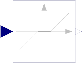 Block Modelica.Blocks.Nonlinear.DeadZone
The DeadZone block defines a region of zero output.
If the input is within uMin ... uMax, the output is zero. Outside of this zone, the output is a linear function of the input with a slope of 1.
Extends from Modelica.Blocks.Interfaces.SISO (Single Input Single Output continuous control block).
| Type | Name | Default | Description |
|---|---|---|---|
Real | uMax | Upper limits of dead zones | |
Real | uMin | -uMax | Lower limits of dead zones |
Boolean | deadZoneAtInit | true | Has no longer an effect and is only kept for backwards compatibility (the implementation uses now the homotopy operator) |
| Type | Name | Description |
|---|---|---|
input RealInput | u | Connector of Real input signal |
output RealOutput | y | Connector of Real output signal |
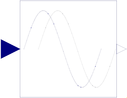 Block Modelica.Blocks.Nonlinear.FixedDelay
The Input signal is delayed by a given time instant, or more precisely:
   y = u(time - delayTime) for time > time.start + delayTime
     = u(time.start)       for time ≤ time.start + delayTime
Extends from Modelica.Blocks.Interfaces.SISO (Single Input Single Output continuous control block).
| Type | Name | Default | Description |
|---|---|---|---|
Time | delayTime | Delay time of output with respect to input signal |
| Type | Name | Description |
|---|---|---|
input RealInput | u | Connector of Real input signal |
output RealOutput | y | Connector of Real output signal |
 Block Modelica.Blocks.Nonlinear.PadeDelay
The Input signal is delayed by a given time instant, or more precisely:
   y = u(time - delayTime) for time > time.start + delayTime
     = u(time.start)       for time ≤ time.start + delayTime
The delay is approximated by a Pade approximation, i.e., by a transfer function
           b[1]*s^m + b[2]*s^[m-1] + ... + b[m+1]
   y(s) = --------------------------------------------- * u(s)
           a[1]*s^n + a[2]*s^[n-1] + ... + a[n+1]
where the coefficients b[:] and a[:] are calculated such that the coefficients of the Taylor expansion of the delay exp(-T*s) around s=0 are identical up to order n+m.
The main advantage of this approach is that the delay is approximated by a linear differential equation system, which is continuous and continuously differentiable. For example, it is uncritical to linearize a system containing a Pade-approximated delay.
The standard text book version uses order "m=n", which is also the default setting of this block. The setting "m=n-1" may yield a better approximation in certain cases.
It is strongly recommended to always set parameter balance = true, in order to arrive at a much better reliable numerical computation. This is not the default, in order to be backwards compatible, so you have to explicitly set it. Besides better numerics, also all states are initialized with balance = true (in steady-state, so der(x)=0). Longer explanation:
By default the transfer function of the Pade approximation is implemented in controller canonical form. This results in coefficients of the A-matrix in the order of 1 up to the order of O(1/delayTime)^n. For already modest values of delayTime and n, this gives largely varying coefficients (for example delayTime=0.001 and n=4 results in coefficients between 1 and 1e12). In turn, this results in a large norm of the system matrix [A,B;C,D] and therefore in unreliable numerical computations. When setting parameter balance = true, a state transformation is performed that considerably reduces the norm of the system matrix. This is performed without introducing round-off errors. For details see function balanceABC. As a result, both the simulation of the PadeDelay block, and especially its linearization becomes more reliable.
Otto Foellinger: Regelungstechnik, 8. Auflage, chapter 11.9, page 412-414, Huethig Verlag Heidelberg, 1994
Extends from Modelica.Blocks.Interfaces.SISO (Single Input Single Output continuous control block).
| Type | Name | Default | Description |
|---|---|---|---|
Time | delayTime | Delay time of output with respect to input signal | |
Integer | n | 1 | Order of Pade delay |
Integer | m | n | Order of numerator (usually m=n, or m=n-1) |
Boolean | balance | false | = true, if state space system is balanced (highly recommended), otherwise textbook version |
| Type | Name | Description |
|---|---|---|
input RealInput | u | Connector of Real input signal |
output RealOutput | y | Connector of Real output signal |
 Block Modelica.Blocks.Nonlinear.VariableDelay
The Input signal is delayed by a given time instant, or more precisely:
   y = u(time - delayTime) for time > time.start + delayTime
     = u(time.start)       for time ≤ time.start + delayTime
where delayTime is an additional input signal which must follow the following relationship:
0 ≤ delayTime ≤ delayMax
Extends from Modelica.Blocks.Interfaces.SISO (Single Input Single Output continuous control block).
| Type | Name | Default | Description |
|---|---|---|---|
Duration | delayMax | Maximum delay time |
| Type | Name | Description |
|---|---|---|
input RealInput | u | Connector of Real input signal |
output RealOutput | y | Connector of Real output signal |
input RealInput | delayTime |