Example 1: Getting Started
In this section, a simple example of a Near Field simulation will be shown. This simulation will be performed considering a cube as the geometry. An Ultrasound Source will be defined as an ultrasound pattern file (also called Annex 1: DUS File Format).
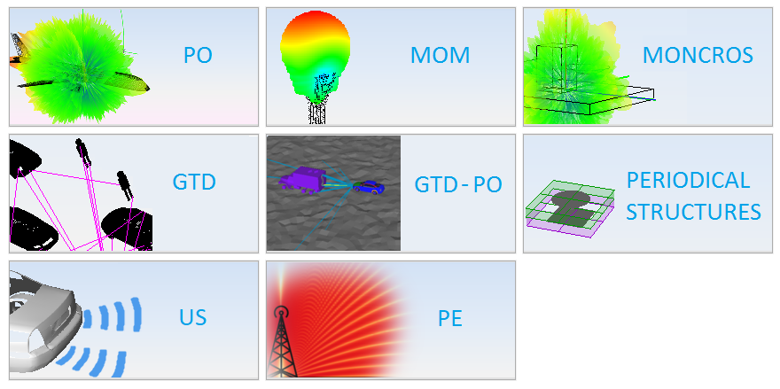
Step 1: The first step consists of creating a new data file where all the parameters of the simulation will be saved. Use the command New from the File menu. Select US type.
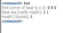
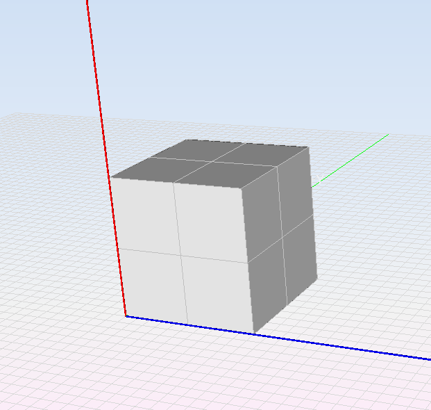
Step 2: The second step is to generate the box. Select GeometrySolid. It will be located at (0,0,0) and the dimensions are 1x1x1 m.
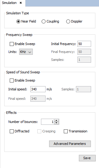
Step 3: The next step is to set the main parameters of the simulations, which are located in .
- Near field in Simulation Type.
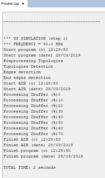
- The number of frequency points and the frequency in this example 1 and 50 kHz.
- The Speed of Sound Sweep will be 340 m/s
- The effect order will be 1.
The rest of the options are the default ones.
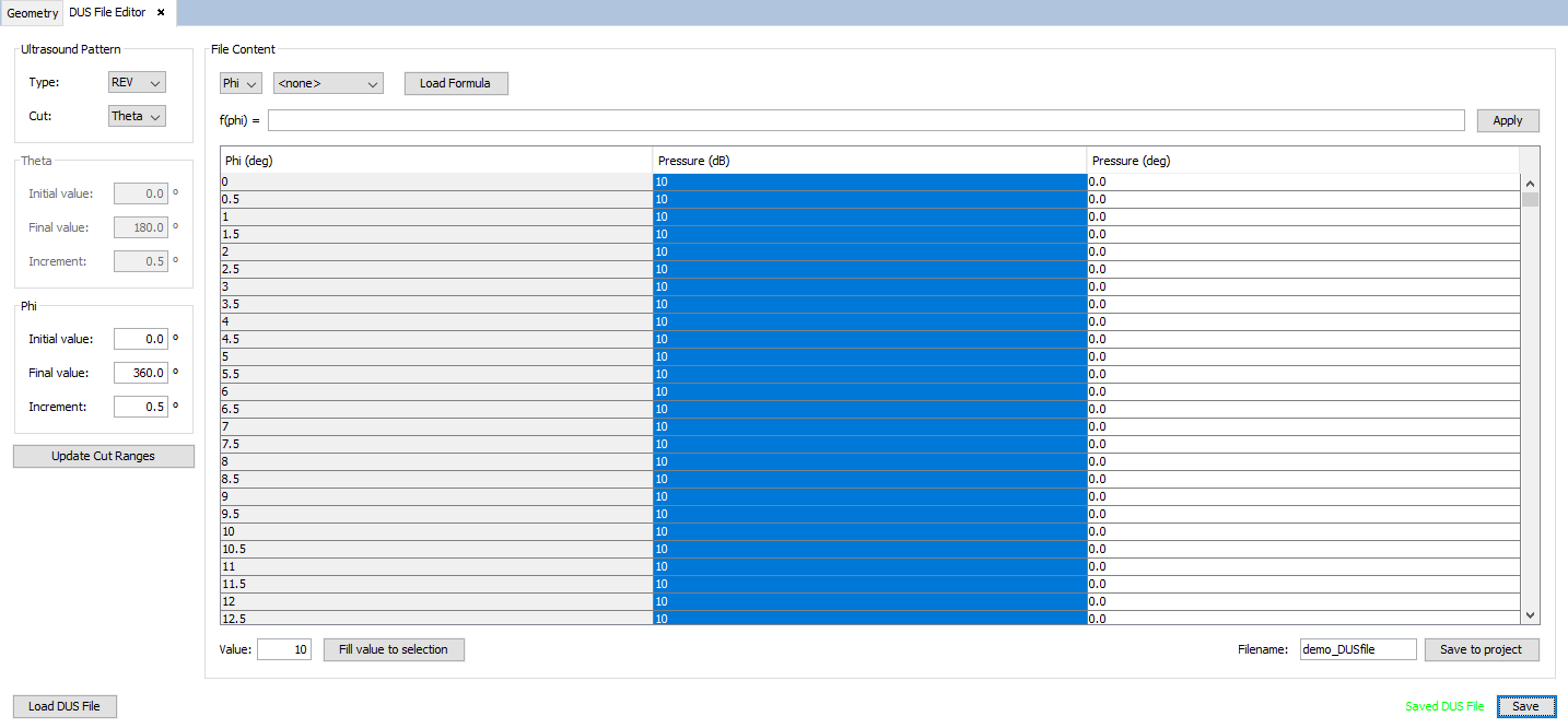
Step 4a: To create a new ultrasound pattern file (.dus), select the Source menu → DUS Source Editor. The user can find more info about DUS Source format at Annex 1: DUS File Format.
In this case, an omnidirectional pattern file has been edited.
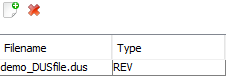
Step 4b: Import the ultrasound pattern (DUS file) to the current project. In this example, the user has to import the demo_DUSfile.dus file.
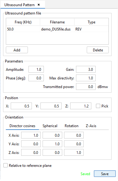
Step 5: Define the position of the ultrasound pattern over the cube clicking on .
Set the ultrasound pattern file. Click on the add button and add the previous imported file.
Set the Amplitude and Phase.
Set the position of the source on (0.5, 0.5, 1.2).
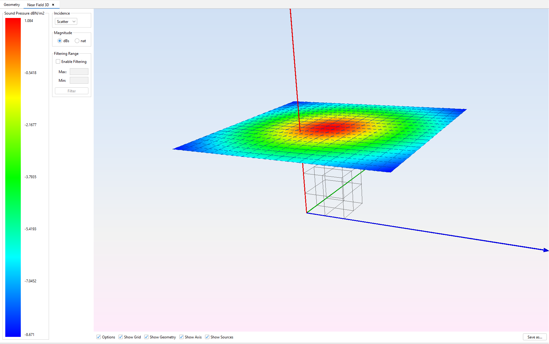
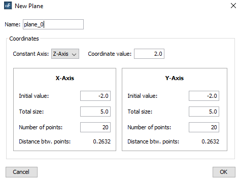
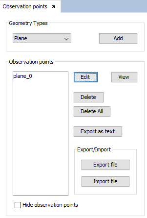
Step 6: The next step is to define the position of the observations points. Select Observation points from Output menu. In Geometry Types dialog, select Plane and click on the Add button.
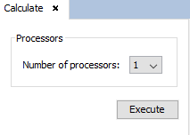
Step 7: To mesh the geometry click on and select the number of processors.
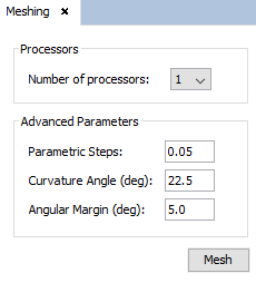
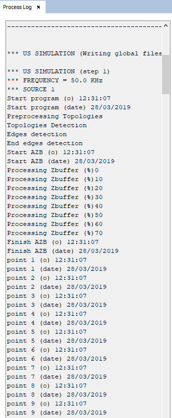
Step 8: Execute the simulation by selecting and introduce the number of processors to be used.
Step 9: After obtaining the results, choose view ray from show results. It is possible to visualize order 1 rays. It is possible to represent the ray tracing interacting with the geometry.
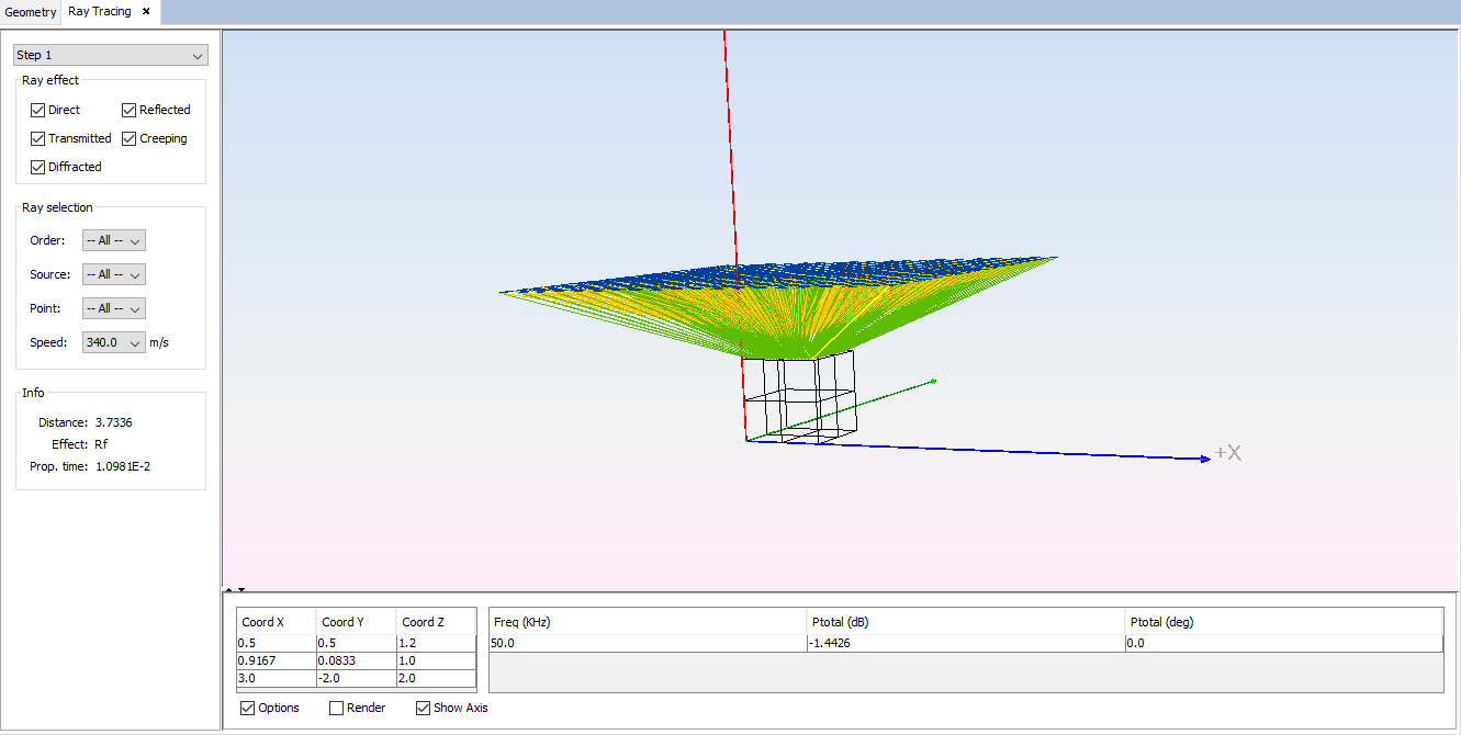
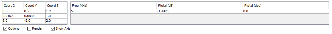
Step 9: It is possible to select a ray to show its information. Clicking in one of the ray will fill its information in the bottom of the panel.
Step 10: To visualize the charts click on , after which the following dialog will be shown: