Test Case B

This example describesthe calculation offield differencein aobservation planeofpointsbetween twoboxeswithoutandwith a slot, having adipoleinone of the boxes. The same processwill be performedon a lineofobservationinside the boxin which thedipoleis not found.

Step 1: Create a new MOM Project.

Open 'New Fasant' and select 'File --> New' option.

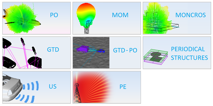
Select 'MOM' option on the previous figure and start to configure the project.

Step 2: Create the geometry model.

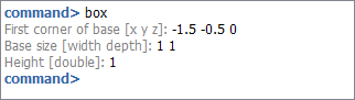
Execute 'box' command writing it on command line and sets the parameters as the next figure shows when command line ask for it.

To generate other box execute 'symmetric' command as the next figure shows.

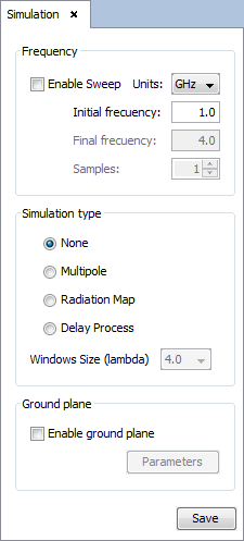
Step 3: Set Simulation Parameters

Select 'Simulation --> Parameters' option on the menu bar and the following panel appears. Set the parameters as the next figure shows and save it.

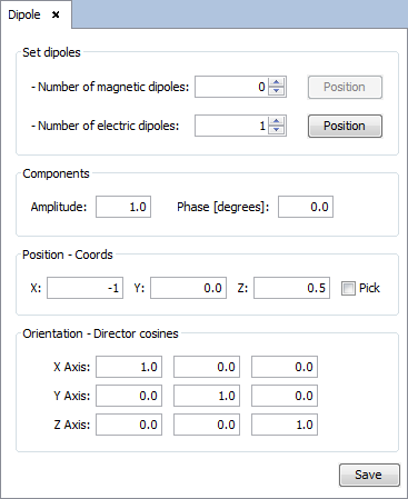
Step 4: Set the antenna parameters.

Select 'Antenna --> Dipole Antenna' option and set the parameters as show the next figure. Then save the parameters and the antenna appears.

Step 5: Set Near Field parameters.

Select 'Output --> Observation Points' option. The following panel will appear.

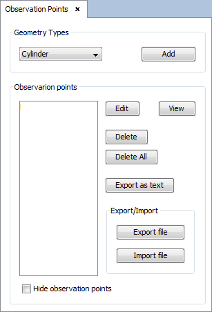
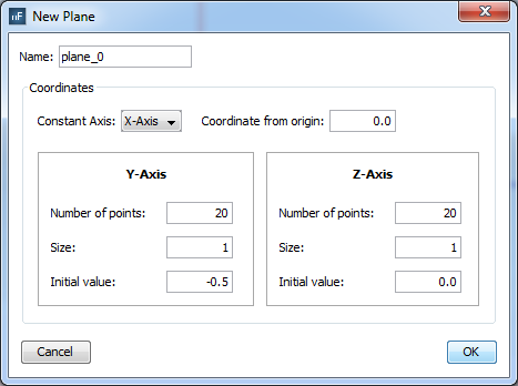
To add a plane visualization, select 'plane' on the selector of 'Geometry Types' section and click on 'Add' button. The plane parameters panel will appear, then configure the values as the next figure show and accept it clicking on 'OK' button.

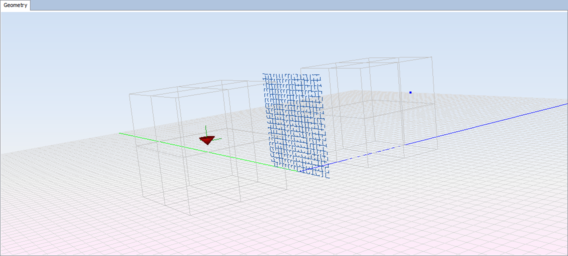
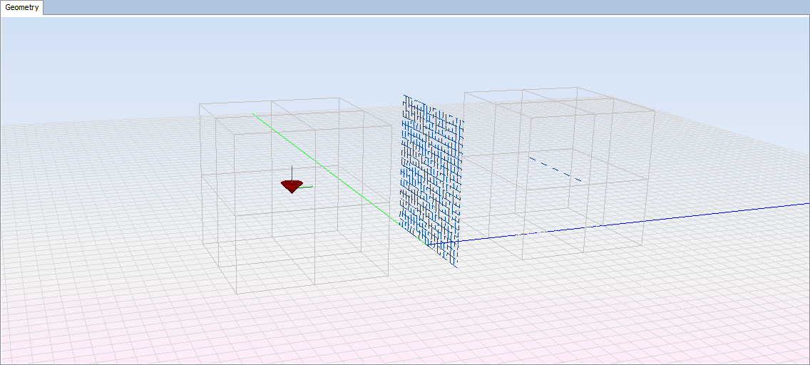
The observation will appear as a dashed line on the position configured.

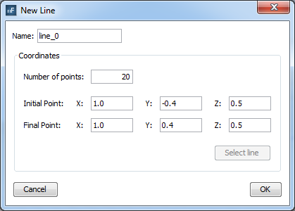
To add the line observation, repeat this step with the 'line' option on the selector of 'Geometry Types' and the following parameters.

Step 6: Meshing the geometry model.

Select 'Meshing --> Parameters' to open the meshing configuration panel and then set the parameters as show the next figure.

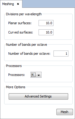
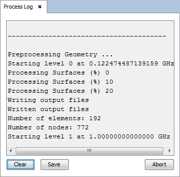
Then click on 'Mesh' button to starting the meshing. A panel appears to display meshing process information.

Step 7: Execute the simulation.

Select 'Calculate --> Execute' option to open simulation parameters. Then select the number of processors as the next figure show.

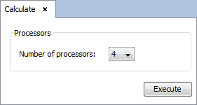
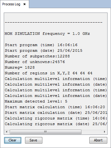
Then click on 'Execute' button to starting the simulation. A panel appears to display execute process information.

Step 8: Save the project

Select 'File --> Save' option to save the project. Select a name and a path to save it on the file chooser that appears.

Step 9: Modify the geometry to make the slots in the boxes.

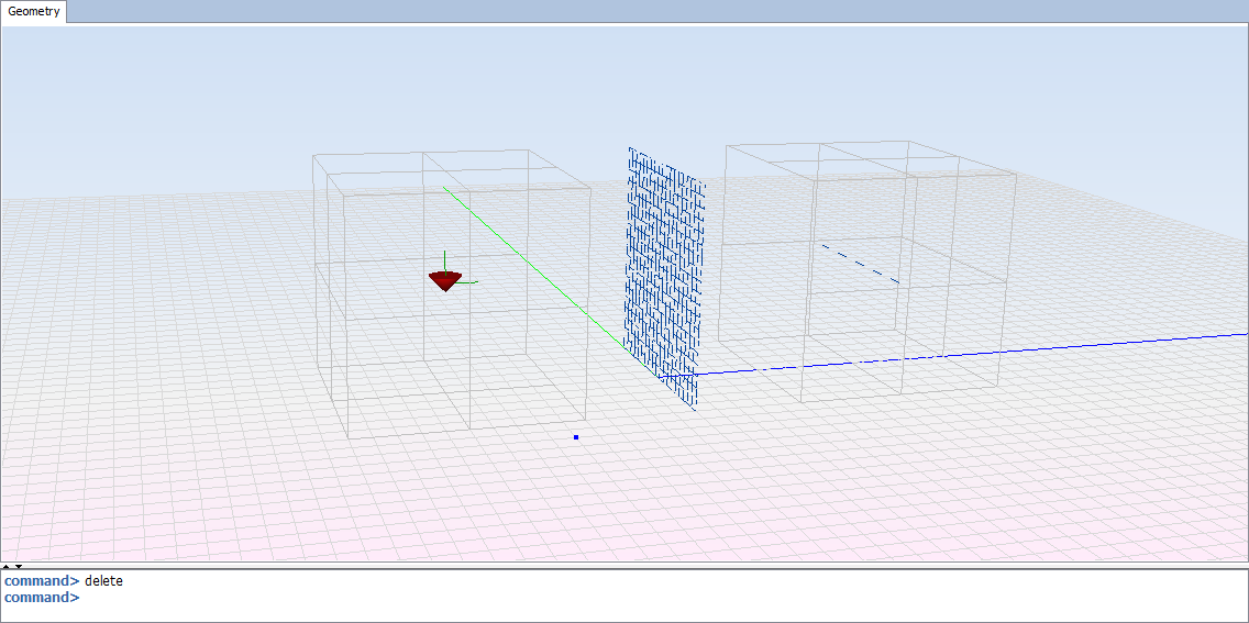
Execute 'explode' command with the boxes selected and follow the steps like shows the next figure. This command divide each object on independent surfaces.

Execute 'delete' command with the nearest surface to observation plane selected in the boxes.

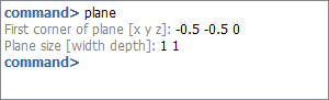
Execute 'plane' command with the parameters shows on the next figure.

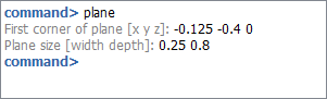
Repeat the operation with the following parameters.

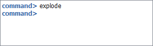
Execute 'explode' command with the new planes selected.

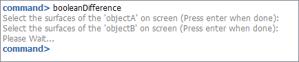
Execute 'booleanDifference' command with the surfaces given for the previous 'explode'. This command ask for two surface to eliminate the second one from the first one.

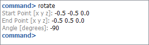
Execute 'rotate' command with the new surface previously selected, using the parameters shown on the next figure.

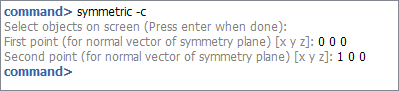
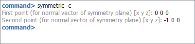
Execute 'symmetric -c' command with the surface used on previous step. Use 'symmetric' parameters as the following figure shows.

Execute 'group' command with the surfaces composing one of the boxes previously selected. Then repeat the operation with the surfaces composing the other box.

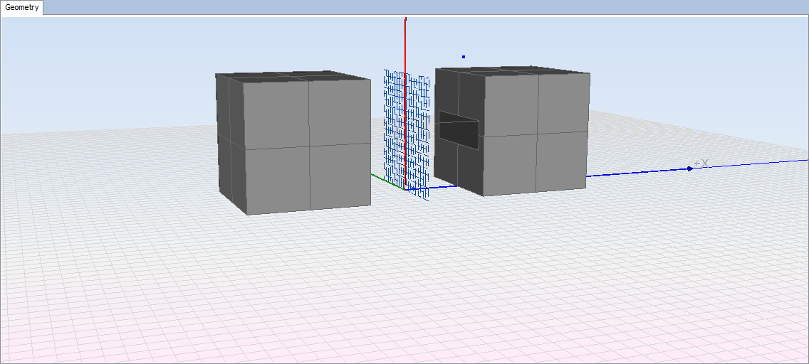
The final result is a geometry with two boxes with a slot on the front surface to the observation plane.

Step 10: Meshing and calculate again like steps 6 and 7.

Step 11: Show results.

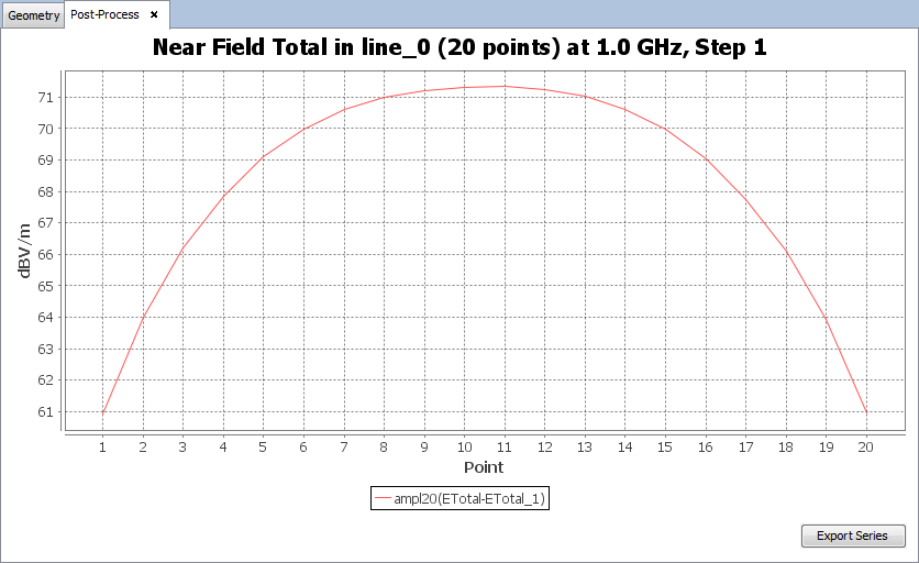
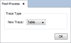
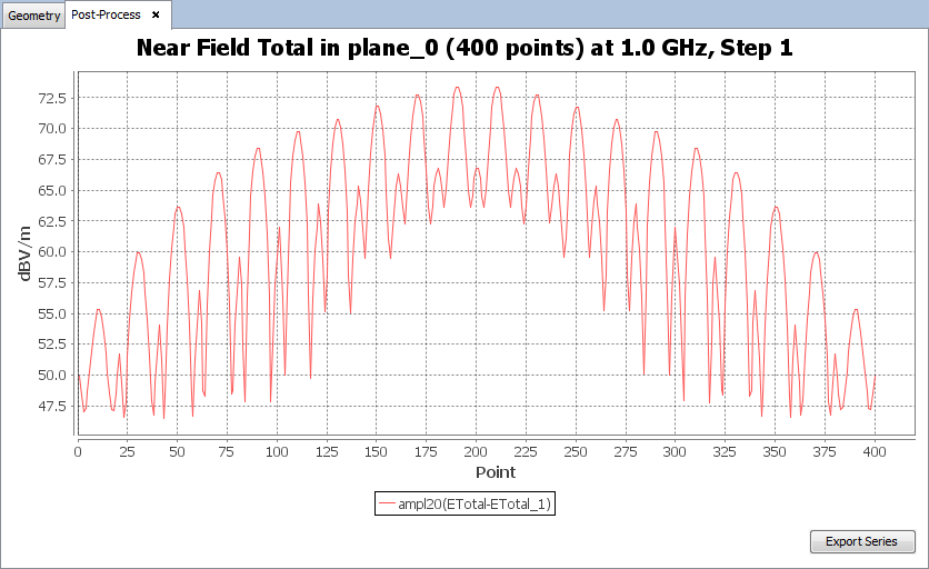
Select 'Show Results --> Post-Process' option to calculate the field difference on the plane observation between this example (slotted boxes) and the example executed on the first part of this guide (closed boxes). To see the result as a plot, select 'plot' on the selector of 'New Trace' option and click on 'OK' button.

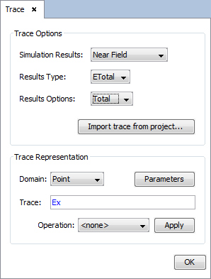
To import the result of the other project, first select the result to show on 'Simulation results', 'Results Type' and 'Results Options' combo boxes. In this case, the values of the next figure for 'Trace options' panel.

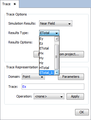
Then click on 'Import trace form project' button to import the selected results to a project. In the panel that appears, select the project on the file chooser opened with 'Browse' button. Then click on 'Save' button to import the results. The imported results appears on 'Results Type' combo box as a new entry with the name of the selected to import with an index indicating the order of the imported projects.

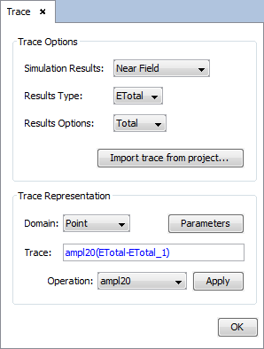
Set the parameters as next figure and add on 'OK' button.

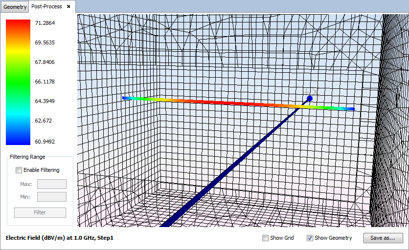
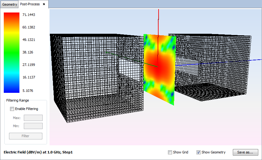
To show the result as a diagram, repeat step 11 selecting 'diagram' on the 'Post-Process Trace' panel.

To show the same results over the line observation, follow the steps explained for the plane observation but previously to click on 'OK' button to show the results, click on 'Parameters' button on 'Trace Representation' panel. Then select the line observation on the panel that appears and confirm the changes.