Advanced Solver Options

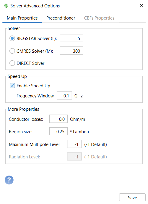
The Main Properties tab looks like this:

• Solver: Three algorithms to solve the problem are available. We can choose between two iterative methods, like BICGSTAB (BiConjugate Gradient STAbilized method) and GMRES (Generalized Minimal Residual method), and the DIRECT solver. If no convergence is achieved by using any of the iterative methods, it is recommended to try to use the other one.
  Note: The direct solution method may require huge memory and time resources when a large number of unknowns is considered.
• Speed Up: If the user enables the speed-up, this option reduces the analysis time for problems that have several frequencies.
• More Properties: The user can specify the next parameters
  • Conductor losses: the metallic structures may induce the conduction losses defined by its parameter, specified in Ohm/m. By default, no conductor losses are considered.
  • Region Size: this parameter defines the size edge (in terms of wavelengths) of the regions generated in the MLFMA-MoM (Multi-Level Fast Multipole Algorithm – Method of Moments) algorithm.
  • Maximum Multipole Level: it is an advanced parameter that defines the maximum number of levels considered in the MLFMA-MoM solver to consider the coupling effect. The default value (-1) consider the coupling in every levels, whereas an integer positive value specifies that the coupling is only considered between the regions up to this level. The more levels consider the coupling effect, the more accurate is the provided solution but also the slower is the solution process. Radiation Level this parameter sets the maximum radiation level in the multipole generation to obtain the radiated fields. The default value (-1) let the program to adjust automatically this configuration. For very large simulations, it may be used to save memory and time resources by avoiding the computation of radiated far field in the largest regions.
  • Compute 3D Pattern: The 3D Pattern is a spherical diagram that shows the field distribution of the analyzed problem. The resolution of the spherical diagram may be modified by the user with the Angle Step parameter (in degrees), that specifies the angular step taken into account in the diagram computation. Disable the Compute 3D Pattern to avoid the 3D Pattern generation whenever it is not required, the simulation time may be reduced.

Preconditioner tab:

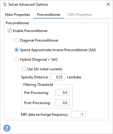
In the subdomains analysis, the user can enable the preconditioner to speed up the resolution of the problem with the Enable Preconditioner option. The user can choose between two different preconditioners:

• Diagonal Preconditioner The diagonal preconditioner is fast to compute and requires a reduced amount of memory, although the improvement in the convergence rate it produces is normally moderate. This preconditioner it is only recommended when more than 8 divisions per wavelength is set in the meshing process, as a shorter number of divisions slows down the convergence instead not using this preconditioner.
• Sparse Approximate Inverse Preconditioner (SAI) This preconditioner will generally result in a faster convergence than the diagonal preconditioner.
  • Use SAI initial currents: This option set the currents computed using the SAI preconditioner as the initial vector of the iterative method. It may be useful if not convergence is achieved in the solution of the problem.
  • Sparsity Distance: This parameter is expressed in wavelengths (0.25 as the default value) and indicates how accurately this preconditioner will resemble the inverse of the rigorous MoM matrix. Higher values will normally involve a faster convergence, but the memory required to store the preconditioner data will grow fast, non-linearly. We advice to keep the default value or increase it slightly in case of specially ill-conditioned systems.
  • Filtering Threshold: These parameters should contain a value between 0.0 and 1.0. The default values should be adequate in most cases.
  • Pre-Processing: This parameter controls the amount of data considered to generate the preconditioner. Lower values entail a more accurate generation, while higher values entail a faster computation.
  • Post-Processing: This parameter controls the amount of data to be stored after the generation of the preconditioner. Lower values entail better convergence, while higher values entail less RAM required to store the preconditioner.
  • MPI Data Exchange Frequency: This parameter sets up how often the MPI nodes request more coupling terms to generate the preconditioner. Larger values require less interactions speeding up the simulation, although more memory will be needed to store these terms. A negative or 0 value indicates that the coupling terms are only exchanged once.
• Hybrid (Diagonal + SAI) : This preconditioner is suited for memory-shared machines, in which case will use both Diagonal and SAI preconditioners.

Due to its numerical nature, the SAI preconditioner is better suited for the case of shared memory parallelization ( OpenMP), while the conventional diagonal preconditioner can be used either for OpenMP or for the MPI paradigm.

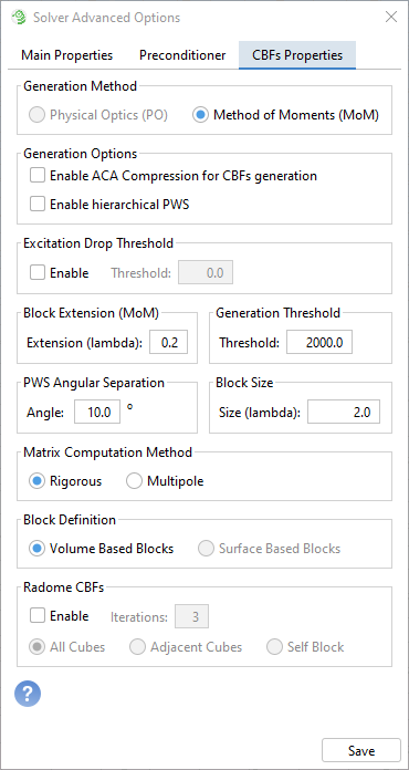
CBFs Propierties tab (available only for antennas with radome structures):

When Macro Basis Functions (CBFs Radome) option is enabled in the panel Solver Functions in the Solver menu, the following options are available as well: