Continuum Analysis

Continuum Analysis allows you to view and analyze your simulation data as a Continuum instead of discrete particles.

Using EDEM Analyst, you can calculate the following Continuum quantities:

Granular temperature
Kinetic pressure
Mass density
Momentum density
Porosity
Solid fraction
Velocity
Shear stress
Normal stress
Concentration
In addition to this, Continuum Analysis can also display EDEM Custom Property data generated through the EDEM API model.

Calculation Methods

For display of Continuum Analysis, a mesh which can be generated from either simple planes or by importing CAD Geometry is required. Particle data is evaluated for each node in the mesh and the coloring can then be applied and smoothed across the mesh.

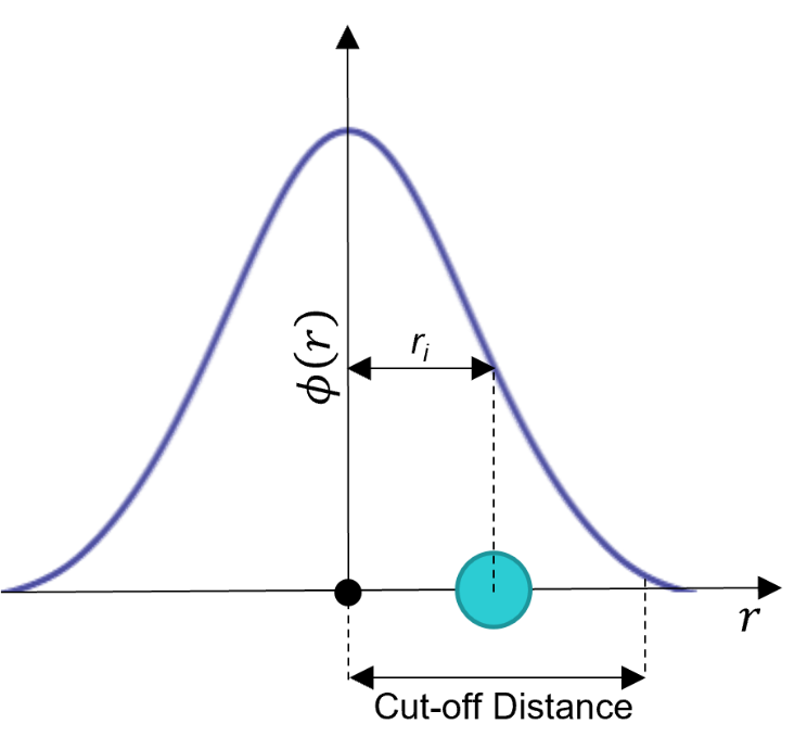
To calculate the Continuum values at each evaluation point, a distance weighted sum of the particle data is performed using the following Gaussian Weighting function where Φ(r) is the Gaussian Distribution function relative to the distance r, a given particle away from a given point.

$ϕ = \frac{1}{\sqrt{{({(\frac{c u t o f f}{3})}^{2} π)}^{\frac{3}{2}}}} e^{- \frac{{|r|}^{2}}{{(\frac{c u t o f f}{3})}^{2}}}$

The cut-off distance is used to determine the width of the distribution function. Using the above equation, 99% of the function's weighting is within a sphere of influence with a radius equal to the cut-off distance. Particles outside the sphere of influence of an evaluation point will not be included in the continuum calculation for that point. This is a parameter that you can change based on their particle data although a value of nine times the average particle diameters is typically recommended, especially if the particle size distribution is narrow.

The following equations are used to extract particle data and apply attribute values to the evaluation points using the Gaussian distribution function.

Mass density

where ρ(r,t) is the mass density, is the mass of the particle, and is the Gaussian function weighting.

$ρ (r, t) = \sum_{i} m_{i} ϕ (r - r_{i})$

Momentum density

The magnitude of the momentum density can be analyzed along with the X, Y, and Z components.

$ρ (r, t) = \sum_{i} m_{i} v_{i} ϕ (r - r_{i})$

Granular temperature

where t_g is the granular temperature, vi(t) is velocity and v(r_i(t),t) is velocity of the particle.

$t g = \frac{1}{3} < \sum_{i} (v_{i} (t) - v {(r_{i} (t), (t))}^{2} >$

Kinetic pressure

where q is the kinetic pressure, ρ is the mass density, and v is the velocity

$q = \frac{1}{2} ρ v^{2}$

Solid Fraction

The solid fraction, Φ, is calculated by dividing the mass density, ρ, by the particle’s solid density, ρ_s.

$ϕ = \frac{ρ}{ρ_{s}}$

Porosity

The porosity is the inverse of the Solid Fraction.

Velocity

The velocity, v(r,t), is calculated by dividing the Momentum density by mass density. The magnitude of the velocity can be analyzed along with the X, Y, and Z components.

$v (r, t) = p (r, t) / ρ (r, t)$

Shear and Normal Stress

Shear: XY, YZ, and ZX Normal: XX, YY, and ZZ‎.

$σ_{c} = \sum_{i} b_{i j} F_{i} ϕ (r - r_{i})$

Concentration

The Concentration of each Particle Type is calculated as:

$c 1 = \frac{ϕ_{1}}{ϕ_{1} + ... + ϕ_{n}}$