Stress and Strain Calculation

The stress and strain for a shell element can be written in vector notation. Each component is a stress or strain feature of the element.

The generalized strain $ε$ can be written as:

${ε} = {e_{x}, e_{y}, e_{x y}, k_{x}, k_{y}, k_{x y}}$

Where,

$e_{i j}$: Membrane strain
$χ_{i j}$: Bending strain or curvature

The generalized stress $\sum$ can be written as:

${\sum} = {N_{x}, N_{y}, N_{x y}, M_{x}, M_{y}, M_{x y}}$

Where,

$N_{x} = \int_{- t / 2}^{t / 2} σ_{x} d z$	$M_{x} = - \int_{- t / 2}^{t / 2} σ_{x} z d z$
$N_{y} = \int_{- t / 2}^{t / 2} σ_{y} d z$	$M_{y} = - \int_{- t / 2}^{t / 2} σ_{y} z d z$
$N_{x y} = \int_{- t / 2}^{t / 2} σ_{x y} d z$	$M_{x y} = - \int_{- t / 2}^{t / 2} σ_{x y} z d z$
$N_{y z} = \int_{- t / 2}^{t / 2} σ_{y z} d z$	$N_{x z} = \int_{- t / 2}^{t / 2} σ_{x z} d z$

Isotropic Linear Elastic Stress Calculation

The stress for an isotropic linear elastic shell for each time increment is computed using:

${\sum^{e l} (t + Δ t)} = {\sum (t)} + L {\dot{ε}} Δ t$

Where,

$L = [\begin{matrix} L_{m} & 0 \\ 0 & L_{b} \end{matrix}]$

$L_{m} = [\begin{matrix} \frac{E t}{1 - v^{2}} & \frac{- v E t}{1 - v^{2}} & 0 \\ \frac{- v E t}{1 - v^{2}} & \frac{E t}{1 - v^{2}} & 0 \\ 0 & 0 & \frac{E t}{1 + v} \end{matrix}]$

$L_{b} = [\begin{matrix} \frac{E t^{3}}{12 (1 - v^{2})} & \frac{- v E t^{3}}{12 (1 - v^{2})} & 0 \\ \frac{- v E t^{3}}{12 (1 - v^{2})} & \frac{E t^{3}}{12 (1 - v^{2})} & 0 \\ 0 & 0 & \frac{E t^{3}}{12 (1 + v)} \end{matrix}]$

$E$: Young's or Elastic modulus
$υ$: Poisson's ratio
$t$: Shell thickness

Isotropic Linear Elastic-Plastic Stress Calculation

An incremental step-by-step method is usually used to resolve the nonlinear problems due to elasto-plastic material behavior. The problem is presented by the resolution of the following equation:

$\dot{σ} = C : (\dot{ε} - {\dot{ε}}_{p})$

$f (σ, σ_{y}) = σ_{e q}^{2} - σ_{y}^{2} = 0; {\dot{σ}}_{y} = H {\dot{ε}}^{p}$

$\dot{f} = 0$

and

${\dot{ε}}_{p} = \frac{\partial f}{\partial σ} \dot{λ}$

$f$ is the yield surface function for plasticity for associative hardening. The equivalent stress $σ_{e q}^{}$ may be expressed in form:

$σ_{e q}^{2} = {σ}^{t} [A] {σ}$

with ${σ} = {\begin{matrix} σ_{x x} \\ σ_{y y} \\ σ_{x y} \end{matrix}}$ and $[A] = [\begin{matrix} 1 & - \frac{1}{2} & 0 \\ - \frac{1}{2} & 1 & 0 \\ 0 & 0 & 3 \end{matrix}]$ for von Mises criteria.

The normality law (Stress and Strain Calculation, Equation 10) for associated plasticity is written as:

${{\dot{ε}}_{p}} = \frac{\partial f}{\partial (σ)} \dot{λ} = 2 [A] {σ} \dot{λ} = \frac{{\dot{ε}}^{p}}{σ_{y}} [A] {σ}$

Where, ${\dot{ε}}^{p}$ is the equivalent plastic deformation.

Stress and Strain Calculation, Equation 7 is written in an incremental form:

${σ}_{n + 1} = {σ}_{n} + {d σ} = {σ}_{n} + [C] ({d ε} - {d ε_{p}}) = {σ^{*}} - \frac{d ε^{p}}{σ_{y}^{n + 1}} [C] [A] {σ}_{n + 1}$

Where, ${σ^{*}}$ represents stress components obtained by an elastic increment and $[C]$ the elastic matrix in plane stress. The equations in Stress and Strain Calculation, Equation 7 to Equation 13 lead to obtain the nonlinear equation:

$f (d ε^{p}) = 0$

that can be resolved by an iterative algorithm as Newton-Raphson method.

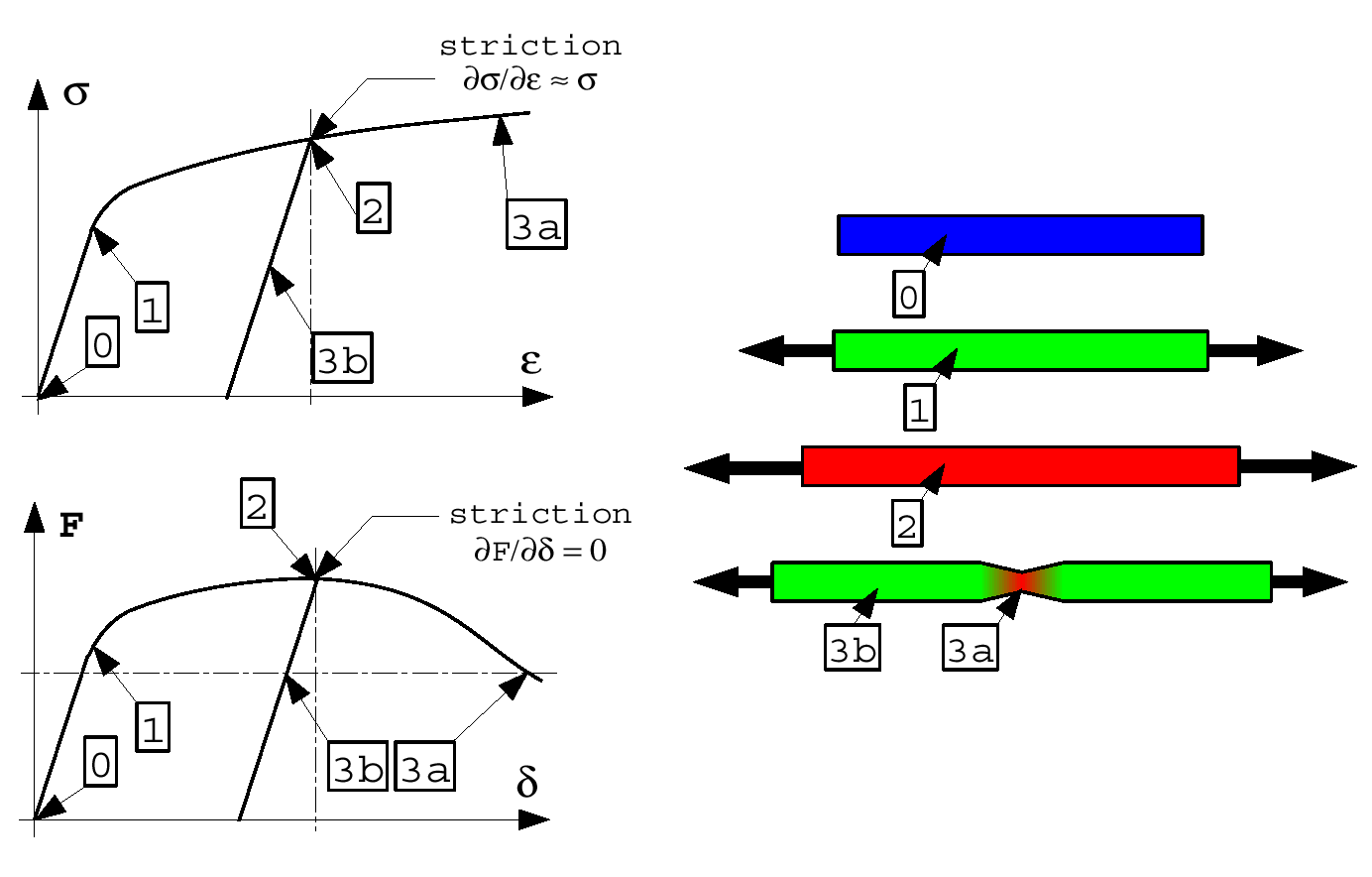
To determine the elastic-plastic state of a shell element, a number of steps have to be performed to check for yielding and defining a plasticity relationship. Stress-strain and force-displacement curves for a particular ductile material are shown in Figure 1.

The steps involved in the stress calculation are:

Strain calculation at integration point z
The overall strain on an element due to both membrane and bending forces is:
$ε_{x} = e_{x} - z χ_{x}$
$ε_{y} = e_{y} - z χ_{y}$
$ε_{x y} = e_{x y} - z χ_{x y}$
${ε} = {ε_{x}, ε_{y}, ε_{x y}}$
Elastic stress calculation
The stress is defined as:
${σ} = {σ_{x}, σ_{y}, σ_{x y}}$
It is calculated using explicit time integration and the strain rate:
${σ^{e l} (t + Δ t)} = {σ (t)} + L {\dot{ε}} Δ t$
$L = [\begin{matrix} \frac{E}{1 - v^{2}} & \frac{v E}{1 - v^{2}} & 0 \\ \frac{v E}{1 - v^{2}} & \frac{E}{1 - v^{2}} & 0 \\ 0 & 0 & \frac{E}{1 + v^{}} \end{matrix}]$
The two shear stresses acting across the thickness of the element are calculated by:
$\begin{array}{l} σ_{y z}^{e l} (t + Δ t) = σ_{y z} (t) + α \frac{E}{1 + v^{}} {\dot{e}}_{y z} Δ t \\ σ_{x z}^{e l} (t + Δ t) = σ_{x z} (t) + α \frac{E}{1 + v^{}} {\dot{e}}_{x z} Δ t \end{array}$
Where, $α$ is the shear factor. Default is Reissner's value of 5/6.
von Mises yield criterion
The von Mises yield criterion for shell elements is defined as:
$σ_{v m}^{2} = σ_{x}^{2} + σ_{y}^{2} - σ_{x}^{} σ_{y}^{} + 3 σ_{x y}^{2}$
For type 2 simple elastic-plastic material, the yield stress is calculated using:
$σ_{y i e l d} (t) = a + b ε^{p^{n}} (t)$
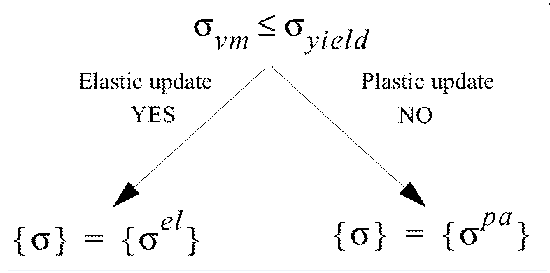
Plasticity Check
The element's state of stress must be checked to see if it has yielded. These values are compared with the von Mises and Yield stresses calculated in the previous step. If the von Mises stress is greater than the yield stress, then the material will be said to be in the plastic range of the stress-strain curve.

Figure 2. Plasticity Check
Compute plastically admissible stresses
If the state of stress of the element is in the plastic region, there are two different analyses that can be used as described in the next paragraph. The scheme used is defined in the shell property set, card 2 of the input.
Compute thickness change
The necking of the shells undergoing large strains in hardening phase can be taken into account by computing normal strain $ε_{z z}$ in an incremental process. The incompressibility hypothesis in plasticity gives:
$d ε_{z z}^{p} = - (d ε_{x x}^{p} + d ε_{y y}^{p})$
Where, the components of membrane strain $d ε_{x x}^{p}$ and $d ε_{y y}^{p}$ are computed by Equation 12 as:
${\begin{array}{l} d ε_{x x}^{p} \\ d ε_{y y}^{p} \end{array}} = \frac{d ε^{p}}{σ_{y}} {[A]}_{2 x 2} {\begin{array}{l} σ_{x x} \\ σ_{y y} \end{array}}$
The plan stress condition $d σ_{z z}^{} = 0$ allows to resolve for $d ε_{z z}^{}$ :
$d ε_{z z} = - \frac{υ}{1 - υ} (d ε_{x x} + d ε_{y y}) + \frac{1 - 2 υ}{1 - υ} d ε_{z z}^{p}$

Plastically Admissible Stresses

Radial return: I_plas=2; When the shell plane stress plasticity flag is set to 0 on card 1 of the shell property type definition, a radial return plasticity analysis is performed. Thus, Step 5 of the stress computation is:; The hardening parameter is calculated using the material stress-strain curve:
$\begin{array}{l} σ_{y i e l d} (t) = a + b ε^{p^{n}} (t) \\ {\dot{ε}}^{p} Δ t = \frac{σ_{v m}^{} - σ_{y i e l d}}{E} \end{array}$; Where, $ε^{p}$ is the plastic strain rate.; The plastic strain, or hardening parameter, is found by explicit time integration:
$ε^{p} (t + Δ t) = ε^{p} (t) + {\dot{ε}}^{p} Δ t$; Finally, the plastic stress is found by the method of radial return. In case of plane stress this method is approximated because it cannot verify simultaneously the plane stress condition and the flow rule. The following return gives a plane stress state:
$σ_{i j}^{p a} = \frac{σ_{y i e l d}}{σ_{v m}^{}} σ_{i j}^{e l}$
Iterative algorithm: I_plas=1; If flag 1 is used on card 1 of the shell property type definition, an incremental method is used. Step 5 is performed using the incremental method described by Mendelson. ^¹ It has been extended to plane stress situations. This method is more computationally expensive, but provides high accuracy on stress distribution, especially when one is interested in residual stress or elastic return. This method is also recommended when variable thickness is being used. After some calculations, the plastic stresses are defined as:
$σ_{x}^{p a} = \frac{σ_{x}^{e l} + σ_{y}^{e l}}{2 (1 + \frac{Δ r}{1 - v})} + \frac{σ_{x}^{e l} - σ_{y}^{e l}}{2 (1 + \frac{3 Δ r}{1 + v})}$
$σ_{y}^{p a} = \frac{σ_{x}^{e l} + σ_{y}^{e l}}{2 (1 + \frac{Δ r}{1 - v})} - \frac{σ_{x}^{e l} - σ_{y}^{e l}}{2 (1 + \frac{3 Δ r}{1 + v})}$
$σ_{x y}^{p a} = \frac{σ_{x y}^{e l}}{1 + \frac{3 Δ r}{1 + v}}$; Where,
$Δ r = \frac{E Δ ε^{p}}{2 σ_{y i e l d} (t + Δ t)}$; The value of $Δ ε^{P}$ must be computed to determine the state of plastic stress. This is done by an iterative method. To calculate the value of $Δ ε^{P}$ , the von Mises yield criterion for the case of plane stress is introduced:
$σ_{x}^{2} + σ_{y}^{2} - σ_{x} σ_{y} + 3 σ_{x y}^{2} = σ_{y i e l d}^{2} (t + Δ t)$; and the values of $σ_{x}$ , $σ_{y}$ , $σ_{xy}$ and $σ_{yield}$ are replaced by their expression as a function of $Δ ε^{P}$ (Hourglass Modes, Equation 1 to Hourglass Modes, Equation 4), with for example:
$σ_{y i e l d}^{} (t + Δ t) = a + b ε^{p^{n}} (t + Δ t)$; and:
$ε^{p^{}} (t + Δ t) = ε^{p^{}} (t) + Δ ε^{p^{}}$; The nonlinear equation Equation 34 is solved iteratively for $Δ ε^{P}$ by Newton's method using three iterations. This is sufficient to obtain $Δ ε^{P}$ accurately.

Plastic Plane Stress with Hill's Criterion

In the case of Hill's orthotropic criterion, the equivalent stress is given by:

$σ_{e q}^{2} = A_{1} σ_{x x}^{2} + A_{2} σ_{y y}^{2} - A_{3} σ_{x x} σ_{y y} + A_{12} σ_{x y}^{2}$

with $[A] = [\begin{matrix} A_{1} & - \frac{A_{3}}{2} & 0 \\ A_{2} & 0 \\ s y m & A_{12} \end{matrix}]$

Equation 13 is then written as:

$[B] {σ}_{n + 1} = {σ^{*}}$

$[B] = [\begin{matrix} 1 + (A_{1} - \frac{A_{3}}{2} υ) d R & (A_{2} υ - \frac{A_{3}}{2}) d R & 0 \\ (A_{1} υ - \frac{A_{3}}{2}) d R & 1 + (A_{2} - \frac{A_{3}}{2} υ) d R & 0 \\ 0 & 0 & 1 + \frac{1 - υ}{2} A_{12} d R \end{matrix}]$ ;

$d R = \frac{d ε^{p}}{σ_{y}} \frac{E}{1 - υ^{2}}$

Changing the stress variables to ${\bar{σ}}$ :

${\bar{σ}} = [Q] {σ}$

with:

$[Q] = [\begin{matrix} 1 & \frac{A_{1} - A_{2} + C}{- 2 (A_{2} υ - \frac{A_{3}}{2})} & 0 \\ \frac{A_{1} - A_{2} + C}{2 (A_{1} υ - \frac{A_{3}}{2})} & 1 & 0 \\ 0 & 0 & 1 \end{matrix}]$ ; $C = \sqrt{(1 - υ^{2}) {(A_{1} - A_{2})}^{2} + {[A_{3} - (A_{1} + A_{2}) υ]}^{2}}$

The matrix $[\bar{B}] = [Q] [B] {[Q]}^{- 1}$ is diagonal:

$[\bar{B}] = [\begin{matrix} 1 + d R (A_{2} - \frac{A_{3} υ}{2} - \frac{C}{J_{Q}}) & 0 & 0 \\ 0 & 1 + d R (A_{1} - \frac{A_{3} υ}{2} + \frac{C}{J_{Q}}) & 0 \\ 0 & 0 & 1 + d R . A_{12} (\frac{1 - υ}{2}) \end{matrix}]$

Where, $J_{Q} = 1 + \frac{{(A_{1} - A_{2} + C)}^{2}}{4 (A_{1} υ - \frac{A_{3}}{2}) (A_{2} υ - \frac{A_{3}}{2})}$ is the Jacobian of [ $Q$ ]. Equation 39 is now written as:

$[\bar{B}] {\bar{σ}}_{n - 1} = {{\bar{σ}}^{*}}$

This will enable to give explicitly the expression of the yield surface Equation 14:

$\begin{array}{l} f_{n + 1} = {(σ_{e q}^{n + 1})}^{2} - {(σ_{y}^{n + 1})}^{2} = {{\bar{σ}}^{*}}^{t} {[\bar{B}]}^{- t} [\bar{A}] {[\bar{B}]}^{- 1} {{\bar{σ}}^{*}} - {(σ_{y}^{n + 1})}^{2} \\ = \frac{{\bar{A}}_{11}}{{\bar{B}}_{1}^{2}} {\bar{σ}}_{x x}^{2} + \frac{{\bar{A}}_{22}}{{\bar{B}}_{2}^{2}} {\bar{σ}}_{y y}^{2} + \frac{A_{12}}{{\bar{B}}_{3}^{2}} {\bar{σ}}_{x y}^{2} + \frac{{\bar{A}}_{12}}{{\bar{B}}_{1} {\bar{B}}_{2}} {\bar{σ}}_{x x} {\bar{σ}}_{y y} - {(σ_{y}^{n + 1})}^{2} \end{array}$

With ${[\bar{A}]}_{2 \times 2} = {[Q]}_{2 \times 2}^{- t} {[A]}_{2 \times 2} {[Q]}_{2 \times 2}^{- 1}$ .

The derivative of $f_{n + 1}$ is carried out in order to use the Newton-Raphson method:

$Δ ε_{n + 1}^{p} = Δ ε_{n}^{p} - \frac{f_{n + 1}}{{f^{'}}_{n + 1}}$

Mendelson A., Plasticity: Theory and Application, MacMillan Co., New York, 1968.