<simulation>
The <simulation> category specifies the main parameters of the simulation like the number of iterations, and the file containing the surface mesh or the fluid material.
<simulation> - <general>
The <general> category contains the following parameters:
- <num_coarsest_iterations>
- Defines the number of iterations at the coarsest refinement level. The physical time per coarsest iteration depends on the material parameters and the Mach factor.
- <mach_factor>
- Default = 1.0
- <parameter_preset>
- This parameter allows you to choose between two presets: default and
fan_noise. Fan noise affects certain parameters differently depending on
the chosen mode and can be initialized to preset. When using the
fan_noise preset, the following settings are automatically changed if
not explicitly specified differently:
- Disable the Cp clipping for all wall models (variants) and outputs.
- Enable raw forces and moments output.
- If seeding is off, set number of ramp-up iterations to 200 (independent of the inlet velocity).
- Local averaging in the OSM region.
- Uniform overset refinement = false.
- Align the moment reference system with the axis of rotation of the first OSM zone.
- Disable sectional drag (current default is 100 sections in x-direction).
- Activate triangulation for section cuts.
- Frozen surface geometry output is activated for full and partial surfaces.
- Far field acoustics parameter is activated.
- <moving_ground>
- The wind tunnel ground is a no-slip wall with zero velocity by default. If it should be moving with <reference_velocity> instead, the parameter must be set to true. If belts are specified (<boundary_conditions>), only the belts will move, not the whole ground.
- <rotating_wheels>
- By specifying this parameter, all rotating boundary conditions (<boundary_conditions>) can be switched on or off at once. If set to false, all entries in the <rotating> category will be effectively ignored.
- <boundary_layer_suction>
- Specifies if a part of the wind tunnel ground starting from the inlet to <boundary_layer_suction_xpos> should be treated as a slip wall, instead of a no-slip wall.
- <boundary_layer_suction_xpos>
- Specifies the x-coordinate (in ), where the slip wall will end, if <boundary_layer_suction> is set to true.
- <reference_velocity>
- The reference velocity (specified in ) is used as velocity at the inlet. It is also used as wall velocity for any belts (if specified) or for the whole wind tunnel ground and for the calculation of the aerodynamic coefficients.
<simulation> - <material>
The <material> category is used to describe the properties of
the fluid material that should be assumed for the simulation, for example, air, and
contains the following parameters:
- <density>
- Density of the material .
- <dynamic_viscosity>
- Dynamic viscosity of the material .
- <temperature>
- Temperature (T) of the material .
- <specific_gas_constant>
- Specific gas constant (R) of the material .
<simulation> - <wall_modeling>
ultraFluidX allows you to specify the handling of near
wall regions of the flow using the following parameters
<coupling>, <wall_model> and
<pressure_gradient>. These parameters can be altered
independently of each other, however certain combinations are not allowed. The
default settings are: <coupling> adaptive_two-way,
<wall_model> GLW and
<pressure_gradient> adverse.
- <coupling> (adaptive_two-way, two-way,one-way, off) default: adaptive_two-way
- This parameter exposes coupling options of how to impose wall shear
stress with the velocity at a donor node, given by the LES computation.
Further past the region, the IBB wall boundary condition is updated with
a slip velocity that enforces the target wall shear stress. This wall
shear stress is calculated by supposing that the donor velocity away
from the wall verifies a given theoretical law of the wall, for example,
like the classical log law; see the <wall_model>
parameter below. Different choices for this coupling are available in
ultraFluidX:
- adaptive_two-way (default)
- GLW is the default law of the wall for this coupling method. The adaptive two way wall-LES coupling model imposes the right near wall slope of velocity as well as the right wall eddy viscosity based on the different information collected in the wall vicinity and the chosen law of the wall. This is the latest coupling model. If adaptive_two-way is specified, the bounding walls (excluding inlet and outlet) are automatically defined as link-based (link_based_bc).
- two-way
- GWF is the default law of the wall for this coupling method. The wall shear stress determined using the wall model is used as an input value for the computation of the slip velocity at the wall.
- one-way
- GWF is the default law of the wall for this coupling method. The slip velocity at the wall is not derived via the wall shear stress. It is based on information at the donor position and coming from the LES in the bulk flow and is directly proportional to this value (non-homogeneous Dirichlet for the velocity). The wall shear stress determined by this coupling approach is computed a posteriori, for instance to be used for the estimation of the viscous force contribution.
- off
- No wall model is used with this parameter. It falls back to the classical no-slip boundary condition (homogeneous Dirichlet for the velocity). The wall shear stress determined by this coupling approach is computed a posteriori, only to be used for the estimation of the viscous force contribution.
- <wall_model> (GLW, GWF, WangMoin, off) default: GLW
- This parameter specifies which theoretical law of the wall should be
used in conjunction with adaptive_two-way or two-way coupling methods in
order to perform an actual Wall Modeled Large Eddy Simulation (WMLES).
Available options:
- GLW (default)
- The generalized law of the wall is a continuous function of + and of the streamwise pressure gradient (adverse only, <pressure_gradient> is automatically set to adverse; the only other option is off.) It has the correct trend for small +; a fine enough mesh is necessary to capture this region correctly. More details are given in reference [1] and [2] .
- GWF
- The Generalized wall function is a set of two piecewise-defined functions, one depending on + and the other depending on c where the velocity scale is a mix of the friction velocity and a velocity scale based on the full pressure gradient (<pressure_gradient> is automatically set to adverse; favorable, adverse and off are the alternative options.) More details are given in reference [3].
- WangMoin
- The law of the wall function is not given explicitly but rather a simplified turbulent boundary layer equation (TBLE) where a given pressure gradient is solved for. More details are given in reference [4] and [5].
- off
- <pressure_gradient> (favorable, adverse, full, off)
- This parameter specifies the way in which pressure gradients along the
wall should be considered by the wall model.
- off
- The wall model will not consider pressure gradients present in the mean flow field and determine the wall shear stress neglecting the respective pressure-gradient term.
- favorable
- The wall model will consider negative pressure gradients in direction of the flow.
- adverse (default)
- The wall model will consider negative and positive pressure gradients in direction of the flow.
- full
- Takes any pressure gradient near the wall into account.
The acceptable combinations when using the various coupling methods are shown below.
The shaded blue boxes indicate default combinations. The line indicates the allowed
combination.
- Adaptive Two-Way Coupling (default)
-
Figure 1. 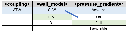
- Two-way coupling
-
Figure 2. 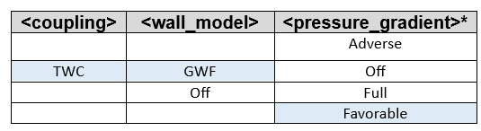
- One-way coupling
-
Figure 3. 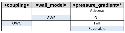
- Coupling off
-
Figure 4. 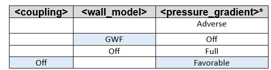
<simulation> - <wall_model_variant>
Different wall model settings apart from the global default (specified via <simulation> - <wall_modeling>) can be set on different parts of the vehicle.
For this purpose, an arbitrary number of such different wall model settings can be
specified as children of <wall_model_variant> via
<wall_model_variant_instance>, each with the following parameters:
- <name>
- Name of the instance, so that it can be referenced in the respective <rotating_instance> or <static_instance> to which it should be applied (mandatory).
- <wall_model> (GLW, GWF, WangMoin, off)
- See above in <simulation> - <wall_modeling>.
- <coupling> (adaptive_two-way, two-way, one-way, off)
- See above in <simulation> - <wall_modeling>.
- <pressure_gradient> (favorable, adverse, full, off)
- See above in <simulation> - <wall_modeling>.
Note: The use of wall model variants is currently not
supported in overset mesh regions. The wall model within the overset regions is
globally specified in <simulation> -
<wall_modeling>.
1 Shih, T. H., Povinelli, L. A., & Liu, N. S.
(2003). Application of generalized wall function for complex turbulent flows.
Journal of Turbulence, 4, 015
2 Wang, M., & Moin, P. (2002). Dynamic wall
modeling for large-eddy simulation of complex turbulent flows. Physics of
Fluids, 14(7), 2043-2051
3 E. Lévêque, H. Touil,
S. Malik, D. Ricot and A. Sengissen, "Wall-modeled large-eddy simulation of the
flow past a rod-airfoil tandem by the Lattice Boltzmann method," International
Journal of Numerical Methods for Heat and Fluid Flow, vol. 28, p. 1096–1116,
2018.
4 J. Boudet, E. Lévêque
and H. Touil, "Unsteady Lattice Boltzmann Simulations of Corner Separation in a
Compressor Cascade," Journal of Turbomachinery, vol. 144, September
2021.
5 T.-H. Shih, L.
Povinelli and N.-S. Liu, "Application of generalized wall function for complex
turbulent flows," vol. 4, Informa UK Limited, 2003.
6 W. Cabot and P. Moin,
"Approximate Wall Boundary Conditions in the Large-Eddy Simulation of High
Reynolds Number Flow," Flow, Turbulence and Combustion, vol. 63, p. 269–291,
2000.
7 M. Wang and P. Moin,
"Dynamic wall modeling for large-eddy simulation of complex turbulent flows,"
Physics of Fluids, vol. 14, p. 2043–2051, 2002.