
A root locus plot computes the locus of closed-loop poles for a transfer function while it’s under gain feedback. The built-in auto-range capability determines the appropriate dynamic range of interest for performing the gain sweep. The number of steps in the sweep determines the number of points in the root locus plot.
For brevity, the transfer function can be denoted as GH(s), which represents a ratio of polynomials in s, and can be written as:
where N(s) is the numerator polynomial and D(s) is the denominator polynomial. The root locus gain is represented as K.
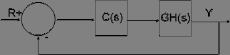
The following diagram presents the structure Embed uses to perform root locus calculations:

The closed-loop poles are the roots of the characteristic equation (or denominator of the closed-loop transfer function) and can be computed as the roots of:
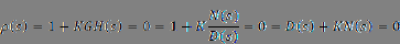
For small values of K, the closed-loop poles are approximately the roots of D(s) = 0 (the open-loop poles); and for large values of K (positive or negative), the closed-loop poles are approximately the roots of N(s) = 0 (the open-loop 0s). The root locus plot presents the paths of the closed-loop poles as the value of K varies.
To generate a root locus plot
1. Prepare the system for linearization.
2. Choose Analyze > Root Locus Options to define the point count resolution of the root locus gain (K) values to be investigated.
3. Choose Analyze > Root Locus to generate a root locus plot.
4. Resize or zoom in on the plot for better viewing.