
Block Category: Signal Consumer
Description: The plot block displays data in a customizable two-dimensional plot. You can customize the plot and control how data is displayed.
Use Edit > Clear Plots/Display to clear the plot.
Memory usage: The plot block uses eight bytes per data point of RAM. If you are running a long simulation at a small step size, it is possible to exceed your RAM limit. For example, a simulation with a step size of 0.005 and duration of 32236 would require 6.4 million points of data per plot trace. At eight bytes per point, each plot trace uses 51MB of RAM. If you used all eight traces on a plot block, you would exceed 412MB of RAM.
Memory usage is calculated at the start of a simulation so you will know immediately if the simulation cannot run due to memory issues.
Basic time domain plots: When you wire a plot block into your diagram and run a simulation, the simulation data is initially presented in time domain. All the signals are plotted on the y-axis; the x-axis represents time. As data points arrive to be plotted, plot bounds are dynamically re-scaled and data points are automatically connected with line segments.
Code generation for plots: If you have a version of Embed that lets you generate code, plot blocks are ignored during code generation.
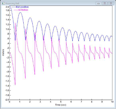
In the above plot, ball position and air friction are displayed as functions of time. The peak ball position follows an exponential decay, governed by air viscosity. The signals are distinguished by line patterns, a feature the plot block automatically performs when displaying or printing on monochrome devices. To make the plot more meaningful, signal labels and a title were also added.
XY plots: In an XY plot, you use one input signal to represent X coordinate generation. As time advances, the remaining input signals are plotted relative to the x-axis signal. To create XY plots, use the XY Plot and X-Axis parameters in the Options dialog.
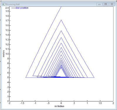
In the XY plot above, ball position is plotted against air friction. At time 0, the ball position is at 2 and air friction is at 0. Over the course of the simulation, the ball position moves counterclockwise, following a three-sided decaying cycle.
To resize plots
You can change the size or shape of the plot block by clicking on the Maximize button in the upper right-hand corner of the plot or dragging its edges or corners.
To zoom in
You can zoom in on plots to view the data at a magnified size. You can zoom in several times in a row for greater magnification. If the area you are zooming in on does not contain at least one data point, the magnified area will be blank.
1. Point to one corner of the area you want to select.
2. To anchor the corner, CTRL+depress.
3. Drag the pointer until the box encloses the area you want to magnify. A status box in the lower left corner of the plot displays the pointer position.
4. Release the button and CTRL key.
To zoom out
•CTRL+right-click the plot.
Printing plots: To print just a plot, click the control-menu box in the upper left corner of the plot and select Print.
Plotting vector data: To plot vector data, use the External Trigger parameter in the Options dialog. This gives you control over when to update vector data.
To save vector data to a file and read it in another application, such as Excel, use the export block.