
Block Category: Integration
Input: Real scalar
Description: The integrator block performs numerical integration on the derivative input signal using the integration algorithm (Euler, trapezoidal, Runge Kutta 2d and 4th orders, adaptive Runge Kutta 5th order, adaptive Bulirsh-Stoer, and backward Euler (Stiff)) selected in the System Properties dialog.
The integrator block is one of the most fundamental and powerful blocks in Embed. This block, together with the limitedIntegrator and resetIntegrator blocks, offer the power to solve an unlimited number of simultaneous linear and nonlinear ordinary differential equations.
You can reset the integrator block to 0 using Reset States.
Code Generation: When generating code for C2000 or ARM Cortex targets and you include one or more integrator blocks in your diagram and you activate Check for Performance Issues in the Code Generation dialog, Embed warns you that large RAM blocks are not supported for the target. You can continue with code generation; however, the generated code may not fit in the target RAM and the code will run slower.
When generating code for Arduino or MSP430 targets, you cannot include integrator blocks in your diagram. Embed halts code generation and issues a message to replace the block.
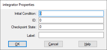
Checkpoint State: Contains the value of the integrator state at the checkpoint. If you have not checkpointed your simulation in System Properties dialog, the value is 0. You can enter a value in hexadecimal notation or as a C expression.
ID: Represents an identification number for the block. It keeps track of the state number that Embed assigns to the integrator. The number of states in any block diagram equals the number of integrators. The default is 0.
Initial Condition: Indicates the initial value of the integrator. The default is 0. You can enter a value in hexadecimal notation or as a C expression.
Label: Indicates a user-defined block label that appears when View > Block Labels is activated.
1. Solving a first order ODE
Consider the simple first order linear differential equation:

where r(t) is an external input. In this case, assume that the external input to the system is a step function. In Embed, such equations are best solved by numerical integration.
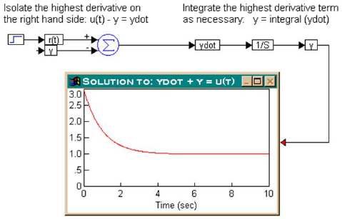
The first step is to isolate the highest derivative term on one side. To understand the procedure better, it is easier to think of isolating the highest derivative term on the right-hand side as:

This equation can be constructed as:
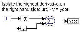
Here, three variable blocks are used for r(t), y, and ydot.
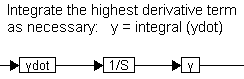
The second step is to integrate the highest derivative term a sufficient number of times to obtain the solution. Since the highest derivative is of first order, ydot must be integrated once to obtain y. This can be realized as:
The overall simulation is shown below.
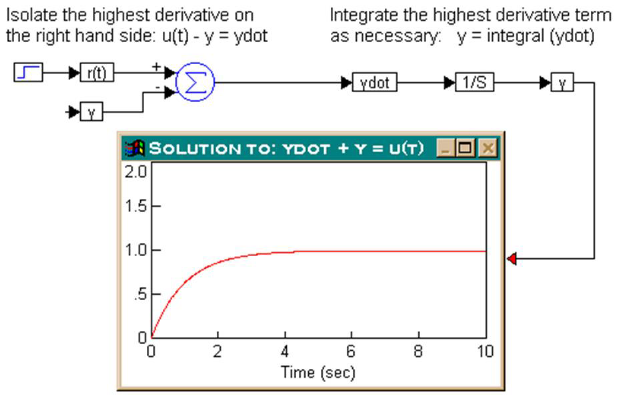
The result shown in the plot block indicates the solution of the differential equation subjected to a step external forcing function.
2. Setting the integrator initial condition internally
Consider the same problem above with the assumption that y(0) = 3. In this case, in addition to the external input r(t), the system response also depends on y(0). This initial condition can be set directly in the integrator block. The result for this case is:
The plot block shows that the response y(t) begins at y(0) = 3 and settles down to 1 for t > 4.5, as expected.
It is important to note that the initial condition on any state (or variable) must be set on the integrator block that is generating that state. (This concept becomes clearer in Example 4.)
3. Setting the integrator initial condition externally
Consider once again the following ordinary differential equation:
Let r(t) be a step function and assume that y(0) = -3.2. The initial condition can be set externally, as shown below.
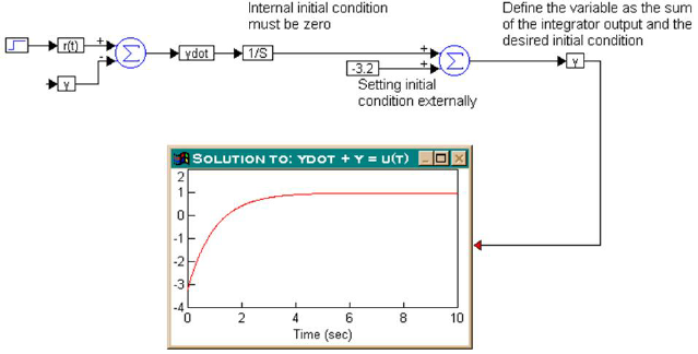
In this configuration, make sure that the internal initial condition of the integrator is set to 0. By default, all integrators have 0 initial condition.
The results indicate that the solution of the ordinary differential equation, subject to the external input and the initial conditions, is computed correctly.
4. Second-order nonlinear ODE with external initial conditions
Consider a second-order nonlinear system given by:
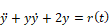
Furthermore, assume that r(t) is a unit step function and that the initial conditions are given by:


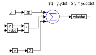
The first step is to isolate the highest derivative term on the right-hand side as:
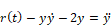
This segment can be coded in Embed as shown below:
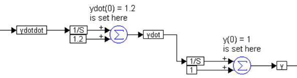
The second step is to integrate ydotdot twice: once to generate ydot, and once more to generate y. As can be imagined, it is crucial to maintain consistent variable names throughout. Furthermore, the initial conditions must be added using the same procedure described in Example 3. This segment can be realized as:
The complete solution for this problem is given by:
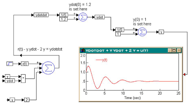
The solution of the equation, y(t) is shown in the plot block.
Note: If you want to use the results of a computational segment in a given diagram as initial conditions for one or more integrators, replace the const blocks with appropriate variable blocks when setting the external initial conditions.