If you create a feedback loop that does not delay, it is referred to as an algebraic loop. When modeling a physical system, the detection of algebraic loops is a gentle warning telling you that you have violated a fundamental law of physics.
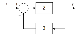
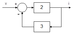
In control theory, the basic structure of a feedback loop in terms of a block diagram is shown below.
For the above structure, the output, y, can be expressed by the mathematical sentence: y is equal to twice the difference of x less three times itself. This sentence can be further reduced to the algebraic expression:

With simple algebraic manipulation, you can easily solve for y in terms of x such that:

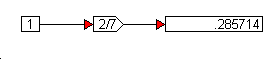
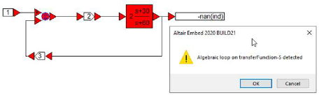
For x=1, you can expect y to be precisely 2/7. You can build this same structure in Embed as shown below:

However, when you start the simulation, Embed immediately reports an algebraic loop.
Perhaps you expected Embed to solve this problem as easily as was done earlier by reducing the system to an algebraic expression and solving as done in the above equations. However, you are working with an algebraic expression, expressed in the form of a feedback loop. You could solve the structure algebraically to get:
And then express this solution in Embed as shown below:
But to solve the original structure requires a different approach that requires you to invoke different tools for solving implicit equations. These will be briefly revisited at the conclusion of this section, but for now let’s dig deeper into the issues of algebraic loops.
Introducing delays to correct algebraic loops
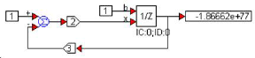
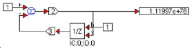
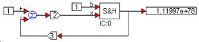
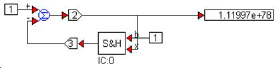
Without further direction, any feedback structure specified in Embed is assumed to be a dynamic structure containing at least one block in the loop that provides memory or equivalently a time delay. Blocks that provide memory include the various integrator blocks, the transferFunction block, unitDelay and timeDelay blocks, sampleHold blocks, buffer blocks, and stateSpace blocks. Revisiting the original feedback loop structure, you can expect to break the algebraic loop by inserting any one of these blocks somewhere in the loop. Below are some examples.
|
Forward Path Delay |
Feedback Path Delay |
|
|
|
|
|
|
|
|
|
|
|
|
In the above examples, completion of the simulation has been accomplished; however, input x=1 is not yielding the expected result for y = 2/7 = 0.285714 as originally obtained. The reason why is because although Embed’s requirement to break the algebraic loop was satisfied, the dynamics towards the correct algebraic solution have been violated:
•In some cases, an unstable response was created that prevented convergence.
•In others, the correct solution was obtained; however, the dynamics that were chosen were inappropriate for the time of simulation.
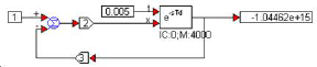
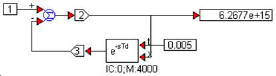
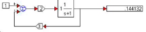
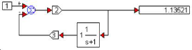
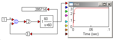
For the latter, let’s examine what’s going on in the following diagram:
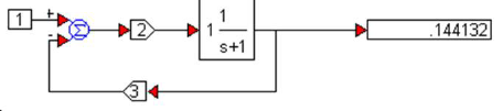
If you plot the result over the simulation time, you see that the output appears to be heading towards the right solution:
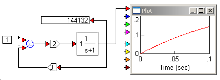
The problem is you either need to increase the simulation end time or change the pole in the transferFunction block to provide faster convergence. Choosing the latter, confirms this expectation:
You can confirm these results by running your own simulation using RK2 integration, a step size of 0.001 and a simulation end time of 0.1 sec.
So far, you have seen how to break the algebraic loop and how to choose and configure an appropriate memory block to arrive at the right answer. This is fine for solving mathematical expressions, but to model a physical system, you need to take a harder look at the physics involved rather than arbitrarily inserting a memory block to satisfy Embed. Remember that the warning of an algebraic loop indicates you have somehow violated a physical law. You need to focus specifically on this violation.
Modeling a physical system with feedback
Assume that in the model of the basic structure of a feedback loop, the factor of 2 and the preceding summingJunction block represent a current feedback amplifier with a transimpedance gain of 2/7, as shown below.
In this model, the factor of 3 represents a 3 Ohm resistive load. Mathematically, the model is no different than the model considered earlier; however, it is now being interpreted as a physical system. The variable y has become the current through a 3 Ohm load and x is the input control voltage. The feedback from the load represents the sensed current in terms of a voltage.
You can expect actual physical systems to behave according to fundamental laws of physics. Regarding the issue of algebraic loops, you need to understand the fundamental law of causality. For strict causality, you not only expect a temporal order of cause and effect, but also a delay in time and space. Newton’s first law says for every action you can expect an opposite and equal reaction, but the second law further says it’s going to take time for the reaction to occur because of inertia. The second law limits bandwidth or the rate at which you can transfer information.
With respect to the amplifier in the above diagram, by expressing the amplifier’s behavior using a simple voltage gain you have ignored the fact that the amplifier has limited bandwidth. The amplifier’s ability to sense the feedback from its load and input command, and respond with a current output is limited in time by the flow of electrons and the impedance to current flow. The model is missing these fundamental attributes and therefore the algebraic loop has occurred.
If the amplifier has a bandwidth of 60 rad/sec, you can represent it as a single pole (lag filter), as done earlier.
By introducing this filter in series with the gain and running the simulation, the algebraic loop is removed, a solution is obtained, and the dynamic features of the amplifier are embedded into the model.
Using a unity gain lead-lag filter
If you assume a unity gain lead-lag filter rather than a lag, the following occurs when you simulate the model:
Here, the lead lag brings back the warning of an algebraic loop. Is this just a bug? No. You must be careful about the structure of the transfer function you choose to break algebraic loops.
The lead-lag filter not strictly causal as illustrated by the following diagram derived from the selected filter.
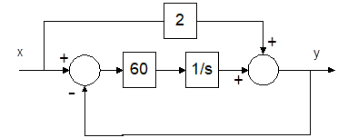
In the structure of the lead-lag filter, you see that there is a path where the input propagates directly to the output with a gain of 2, but without any delay. This forward path leads to the algebraic loop when you connect the filter into a feedback loop that is free of blocks with memory.
In the lead-lag filter diagram, the lead-lag filter is expressed by the transfer function:

In linear control theory, the relative degree of this transfer function is 0. Relative degree is a measure of the difference between the orders of the denominator and numerator polynomials.
For relative degree of 1 or greater, a transfer function is called strictly proper. For relative degree of 0, a transfer function is proper. For relative degree less than 0, a transfer function is improper. These terms are synonymous with causality according to the following table, which also indicates realizability. To realize a linear transfer function, it should be free of derivatives. In other words, it should not be trying to predict the future: that’s a violation of causality.
Strictly Proper → Strictly Causal →Realizable
Proper → Causal →Realizable
Improper →Anti-Causal →Unrealizable
To avoid algebraic loops using linear transfer functions, you need to make sure the transfer function in the loop is always strictly proper.
In the lead-lag filter, and assuming it is implemented by a real physical device (op-amp circuit for example), one additional detail was overlooked: the limited bandwidth of its amplifier. By adding an additional pole to the model, you increase the relative degree to 1 and prevent the algebraic loop from occurring. But more important, you have considered dynamics that more closely approximate reality.
In summary, real physical systems are bound by limitations on bandwidth. This is because all real physical systems impede the propagation of information. Regardless of the technology used, information cannot be transmitted instantaneously. Even optical feedback systems are limited - by the speed of light. Therefore, the choice of all physical models used in feedback system simulations need to be strictly causal or for linear systems strictly proper.
Solving an algebraic system with feedback
You can abandon the realm of physical systems and seek to solve an algebraic system using feedback. Here you are asking the system to solve a mathematical expression possibly without any connection to reality. Fortunately, Newton again offers us a method, as does Embed. Newton’s method and other methods of numerical iteration allow you to solve both linear and nonlinear algebraic equations algorithmically. Embed supports these methods, but you must let it know this is the goal of your diagram. To learn more about numerical solutions of equations in Embed and algebraic loops, see Solving implicit equations.