 Package Modelica.Mechanics.MultiBody.UsersGuide.Tutorial.LoopStructures
Loop structures
Package Modelica.Mechanics.MultiBody.UsersGuide.Tutorial.LoopStructures
The MultiBody library has the feature that all components can be connected together in a nearly arbitrary fashion. Therefore, kinematic loop structures pose in principal no problems. In this section several examples are given, the special treatment of planar loops is discussed and it is explained how a kinematic loop structure can be modeled such that the occurring non-linear algebraic equation systems are solved analytically. There are the following sub-chapters:
Extends from Modelica.Icons.Information (Icon for general information packages).
| Name | Description |
|---|---|
AnalyticLoopHandling | Analytic loop handling |
Introduction | Introduction |
PlanarLoops | Planar loops |
 Class Modelica.Mechanics.MultiBody.UsersGuide.Tutorial.LoopStructures.Introduction
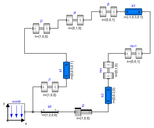
In principal, no special action is needed, if loop structures occur (contrary to the ModelicaAdditions.MultiBody library). An example is presented in the figure below. It is available as MultiBody.Examples.Loops.Fourbar1
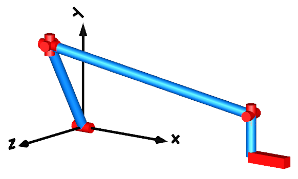
This mechanism consists of 6 revolute joints and 1 prismatic joint and forms a kinematical loop. It has one degree of freedom. In the next figure the default animation is shown. Note, that the axes of the revolute joints are represented by the red cylinders and that the axis of the prismatic joint is represented by the red box on the lower right side.
Whenever loop structures occur, non-linear algebraic equations are present on "position level". It is then usually not possible by structural analysis to select states during translation (which is possible for non-loop structures). In the example above, a non-linear algebraic loop of 54 equations can be detected and reduced to a system of 6 coupled algebraic equations. Note, that this is performed without using any "cut-joints" as it is usually done in multi-body programs, but by just appropriate symbolic equation manipulation. Via the dynamic dummy derivative method the generalized coordinates on position and velocity level from one of the 7 joints are dynamically selected as states during simulation. Whenever, these two states are no longer appropriate, states from one of the other joints are selected during simulation.
The efficiency of loop structures can usually be enhanced, if states are statically fixed at translation time. For this mechanism, the generalized coordinates of joint j1 (i.e., the rotation angle of the revolute joint and its derivative; the joint is visualized as a red cylinder at the x-axis in the animation figure above) can always be used as states. In the abovementioned example, this is already stated by setting parameter "stateSelect = StateSelect.always" in the "Advanced" menu of that joint. When setting this flag for joint j1 in that way in the four bar mechanism, a non-linear algebraic loop of 40 equations can be detected and reduced to a system of 5 coupled non-linear algebraic equations.
In many mechanisms it is possible to solve the non-linear algebraic equations analytically. For a certain class of systems this can be performed also with the MultiBody library. This technique is described in section "Analytic loop handling".
Extends from Modelica.Icons.Information (Icon for general information packages).
 Class Modelica.Mechanics.MultiBody.UsersGuide.Tutorial.LoopStructures.PlanarLoops
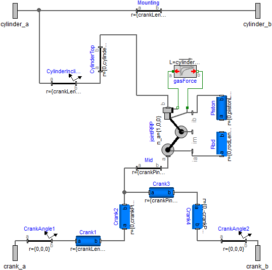
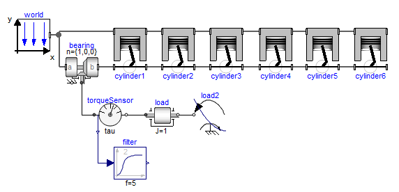
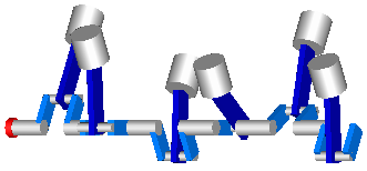
In the figure below, the model of a V6 engine is shown that has a simple combustion model. It is available as MultiBody.Examples.Loops.EngineV6.
The Modelica schematic of one cylinder is given in the figure below. Connecting 6 instances of this cylinder appropriately together results in the engine schematic displayed above.
In the next figure the animation of the engine is shown. Every cylinder consists essentially of 1 prismatic and 2 revolute joints that form a planar loop, since the axes of the two revolute joints are parallel to each other and the axis of the prismatic joint is orthogonal to the revolute joint axes. All 6 cylinders together form a coupled set of 6 loops that have together 1 degree of freedom.
All planar loops, and especially the engine, result in a DAE (= Differential-Algebraic Equation system) that does not have a unique solution. The reason is that, e.g., the cut forces in direction of the axes of the revolute joints cannot be uniquely computed. Any value fulfills the DAE equations. This is a structural property that is determined by the symbolic algorithms. Since they detect that the DAE is structurally singular, a further processing is not possible. Without additional information it is also impossible that the symbolic algorithms could be enhanced because if the axes of rotations of the revolute joints are only slightly changed such that they are no longer parallel to each other, the planar loop can no longer move and has 0 degrees of freedom. Algorithms based on pure structural information cannot distinguish these two cases.
The usual remedy is to remove superfluous constraints, e.g., along the axis of rotation of one revolute joint. Since this is not easy for an inexperienced modeler, the special joint: RevolutePlanarLoopConstraint is provided that removes these constraints. Exactly one revolute joint in a every planar loop must be replaced by this joint type. In the engine example, this special joint is used for the revolute joint B2 in the cylinder model above. The icon of the joint is slightly different to other revolute joints to visualize this case.
If a modeler is not aware of the problems with planar loops and models them without special consideration, a Modelica translator displays an error message and points out that a planar loop may be the reason and suggests to use the RevolutePlanarLoopConstraint joint. This error message is due to an annotation in the Frame connector.
  connector Frame
     ...
     flow SI.Force f[3] annotation(unassignedMessage="..");
  end Frame;
If no assignment can be found for some forces in a connector, the "unassignedMessage" is displayed. In most cases the reason for this is a planar loop or two joints that constrain the same motion. Both cases are discussed in the error message.
Note, that the non-linear algebraic equations occurring in planar loops can be solved analytically in most cases and therefore it is highly recommended to use the techniques discussed in section "Analytic loop handling" for such systems.
Extends from Modelica.Icons.Information (Icon for general information packages).
 Class Modelica.Mechanics.MultiBody.UsersGuide.Tutorial.LoopStructures.AnalyticLoopHandling
It is well known that the non-linear algebraic equations of most mechanical loops in technical devices can be solved analytically. It is, however, difficult to perform this fully automatically and therefore none of the commercial, general purpose multi-body programs, such as MSC ADAMS, LMS DADS, SIMPACK, have this feature. These programs solve loop structures with pure numerical methods. Multi-body programs that are designed for real-time simulation of the dynamics of specific vehicles, such as ve-DYNA, usually contain manual implementations of a particular multi-body system (the vehicle) where the occurring loops are either analytically solved, if this is possible, or are treated by table look-up where the tables are constructed in a pre-processing phase. Without these features the required real-time capability would be difficult to achieve.
In a series of papers and dissertations Prof. Hiller and his group in Duisburg, Germany, have developed systematic methods to handle mechanical loops analytically, see also MultiBody.UsersGuide.Literature. The "characteristic pair of joints" method basically cuts a loop at two joints and uses geometric invariants to reduce the number of algebraic equations, often down to one equation that can be solved analytically. Also several multi-body codes have been developed that are based on this method, e.g., MOBILE. Besides the very desired feature to solve non-linear algebraic equations analytically, i.e., efficiently and in a robust way, there are several drawbacks: It is difficult to apply this method automatically. Even if this would be possible in a good way, there is always the problem that it cannot be guaranteed that the statically selected states lead to no singularity during simulation. Therefore, the "characteristic pair of joints" method is usually manually applied which requires know-how and experience.
In the MultiBody library, the "characteristic pair of joints" method is supported in a restricted form such that it can be applied also by non-specialists. The idea is to provide aggregations of joints in package MultiBody.Joints.Assemblies as one object that either have 6 degrees of freedom or 3 degrees of freedom (for usage in planar loops).
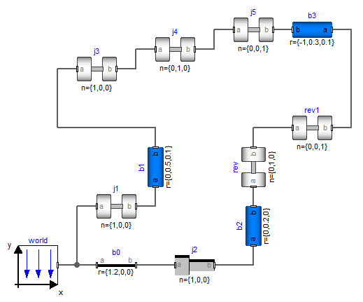
As an example, a variant of the four bar mechanism is given in the figure below.
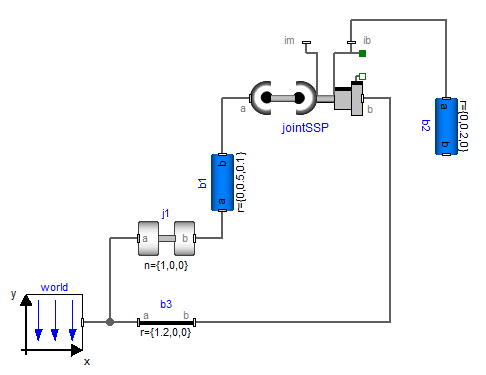
Here, the mechanism is modeled with six revolute joints and one prismatic joint. In the figure below, the five revolute joints and the prismatic joint are collected together in an assembly object called "jointSSP" from MultiBody.Joints.Assemblies.JointSSP.
The JointSSP joint aggregation has a frame at the outer spherical joint (frame_a) and a frame at the prismatic joint (frame_b). JointSSP, as all other objects from the Joints.Assemblies package, has the property, that the generalized coordinates, and all other frames defined in the assembly, can be calculated given the movement of frame_a and of frame_b. This is performed by analytically solving non-linear systems of equations. From a structural point of view, the equations in an assembly object are written in the form
q = f1(ra, Ra, rb, Rb)
where ra, Ra, rb, Rb are the variables defining the position and orientation of the frame_a and frame_b, respectively, and q are the generalized positional coordinates inside the assembly, e.g., the angle of a revolute joint. Given angle j of revolute joint j1 from the four bar mechanism, frame_a and frame_b of the assembly object can be computed by a forward recursion
(ra, Ra, rb, Rb) = f(j)
Since this is a structural property, the symbolic algorithms can automatically select j and its derivative as states and then all positional variables can be computed in a forwards sequence. It is now understandable that a Modelica translator can transform the equations of the four bar mechanism to a recursive sequence of statements that has no non-linear algebraic loops anymore (remember, the previous "straightforward" solution with 6 revolute joints and 1 prismatic joint has a nonlinear system of equations of order 5).
The aggregated joint objects consist of a combination of either a revolute or prismatic joint and of a rod that has either two spherical joints at its two ends or a spherical and a universal joint, respectively. For all combinations, analytic solutions can be determined. For planar loops, combinations of 1, 2 or 3 revolute joints with parallel axes and of 2 or 1 prismatic joint with axes that are orthogonal to the revolute joints can be treated analytically. The currently supported combinations are listed in the table below.
| 3-dimensional Loops: | |
| JointSSR | Spherical - Spherical - Revolute |
| JointSSP | Spherical - Spherical - Prismatic |
| JointUSR | Universal - Spherical - Revolute |
| JointUSP | Universal - Spherical - Prismatic |
| JointUPS | Universal - Prismatic - Spherical |
| Planar Loops: | |
| JointRRR | Revolute - Revolute - Revolute |
| JointRRP | Revolute - Revolute - Prismatic |
On first view this seems to be quite restrictive. However, mechanical devices are usually built up with rods connected by spherical joints on each end, and additionally with revolute and prismatic joints. Therefore, the combinations of the above table occur frequently. The universal joint is usually not present in actual devices but is used (a) if two JointXXX components can be connected such that a revolute and a universal joint together form a spherical joint and (b) if the orientation of the connecting rod between two spherical joints is needed, e.g., since a body shall be attached. In this case one of the spherical joints might be replaced by a universal joint. This approximation is fine as long as the mass and inertia of the rod is not significant.
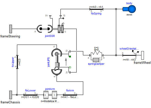
Let us discuss item (a) in more detail: The MacPherson suspension in the next figure has three frame connectors.
The lower left one (frameChassis) is fixed to the vehicle chassis. The upper left one (frameSteering) is driven by the steering mechanism, i.e. the movement of both frames are given. The frame connector on the right (frameWheel) drives the wheel. The three frames are connected by a mechanism consisting essentially of two rods with spherical joints on both ends. These are built up by a jointUPS and a jointSSR assemblies. As can be seen, the universal joint from the jointUPS assembly is connected to the revolute joint of the jointSSR assembly. Therefore, we have 3 revolute joints connected together at one point and if the axes of rotations are chosen appropriately, this describes a spherical joint. In other words, the two connected assemblies define the desired two rods with spherical joints on each ends.
The movement of the chassis, frameChassis, is computed outside of the suspension model. When the generalized coordinates of revolute joint "jointArm" (lower left part in figure) are used as states, then frame_a and frame_b of the jointUPS joint can be calculated. After the non-linear loop with jointUPS is (analytically) solved, all frames on this assembly are known, especially, the one connected to frame_b of the jointSSR assembly. Since frame_a of jointSSR is connected to frameSteering which is computed from the steering mechanism, again the two required frame movements of the jointSSR assembly are calculated. This in turn means that also all other frames on the jointSSR assembly can be computed, especially, the one connected to frameWheel that drives the wheel. From this analysis it is clear that a tool is able to solve these coupled loops analytically.
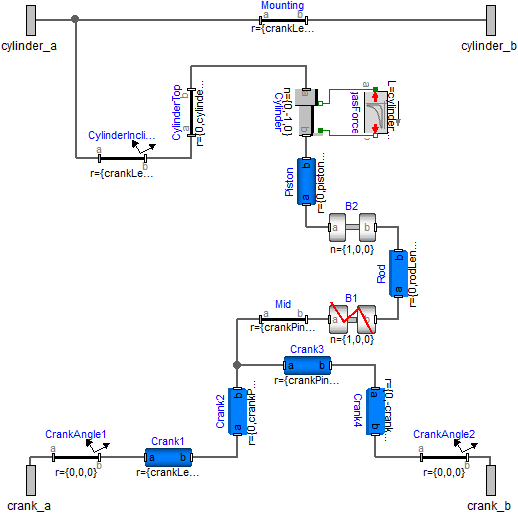
Another example is the model of the V6 engine, see next figure for an animation view and the original definition of one cylinder with elementary joints.
Here, it is sufficient to rewrite the basic cylinder model by replacing the joints with a JointRRP object that has two revolute and one prismatic joint, as can be seen in next figure.
Since 6 cylinders are connected together, 6 coupled loops with 6 JointRRP objects are present. This model is available as MultiBody.Examples.Loops.EngineV6_analytic.
The composition diagram of the connected 6 cylinders is shown in the next figure
It can be seen that the revolute joint of the crank shaft (joint "bearing" in left part of figure) might be selected as degree of freedom. Then, the 4 connector frames of all cylinders can be computed. As a result, the computations of the cylinders are decoupled from each other. Within one cylinder the position of frame_a and frame_b of the jointRRP assembly can be computed and therefore the generalized coordinates of the two revolute and the prismatic joint in the jointRRP object can be determined. Considering this analysis, it is not surprising that a Modelica translator is able to transform the DAE equations into a sequential evaluation without any non-linear loop. Compare this nice result with the model using only elementary joints that leads to a DAE with 6 algebraic loops and 5 non-linear equations per loop. Additionally, a linear system of equations of order 43 is present. The simulation time is about 5 times faster with the analytic loop handling.
Extends from Modelica.Icons.Information (Icon for general information packages).