Example 3: Radiation Pattern File Simulation
In this section, we show how to compute the Near Field using a simple geometry fed by a customized DIA (radiation features definition) file.
Step 1: Create a newFASANT GTD project by selecting the File → New option (or alternatively pressing Ctrl+N) and click on the following icon in the panel:
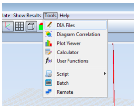
Step 2: To create a new radiation pattern file (.dia), select the Tools –> DIA Files option.
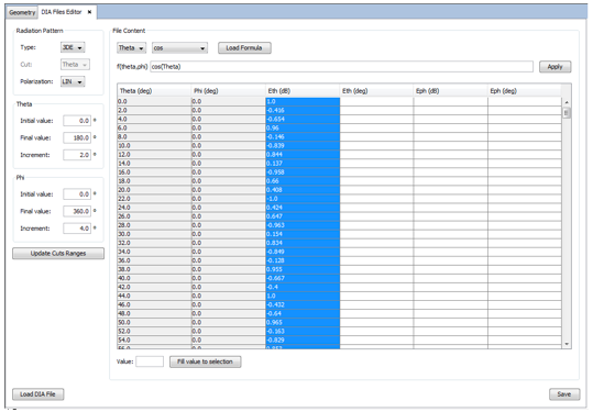
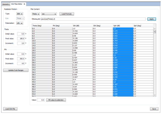
Step 3: Introduce the following parameters in the DIA Files Editor. The formula shown in the first figure has been used to fill the Etheta(dB) column, and the formula is shown in the second figure has been used to fill the Ephi(dB) column.
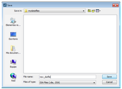
Step 4: Click on the Save button to save the DIA file.
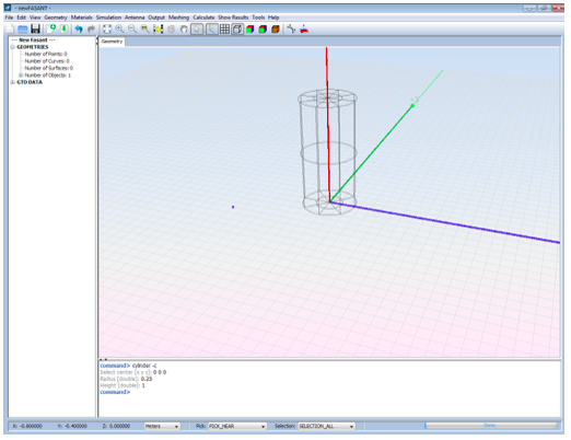
Step 5: Now create the geometry for the simulation. Let’s generate a cylinder using the following command:
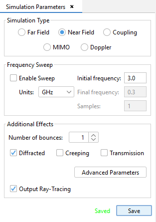
Step 6: Now set up the parameters of the simulation. Select Simulation Parameters → Simulation. Enter the following parameters:
- Near Field simulation type.
- Initial frequency 3.0 GHz. Disable Frequency Sweep.
- Enable diffraction.
- Keep the number of bounces equal to 1.
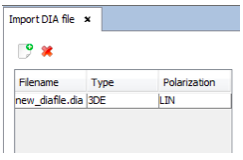
Step 7: Antenna -> Pattern File Antenna -> Import DIA File
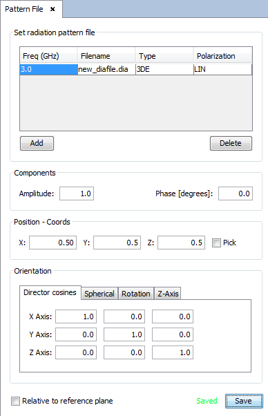
Step 8: Antenna -> Pattern File Antenna -> Pattern File Antenna
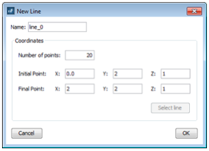
Step 9: Now add a line of observation points. Select the Output → Observation Points option. In the Geometry Types combo box, select Line and press the Add button. The following dialog will pop up. Set the line parameters as shown in the figure.
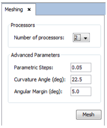
Step 10: Select Meshing → Create Visibility Matrix to mesh. Select the number of processors to use for the meshing process and press the Mesh button.
Step 11: Once the meshing process has finished, run the simulation. To do this, select Calculate → Execute, select the number of processors to use (like we did before meshing) and press the Execute button.
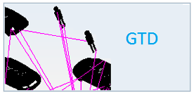
Step 12: When the calculation has finished, press Show Results → View Ray. On the left side of the Ray Visualization panel, select Step 2. The result should be the same as in the following figure:
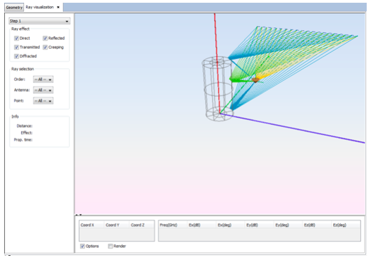
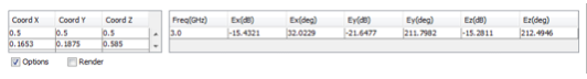
Step 13: It is possible to select a ray to show its information. Clicking in one of the rays will fill its information in the bottom of the panel.
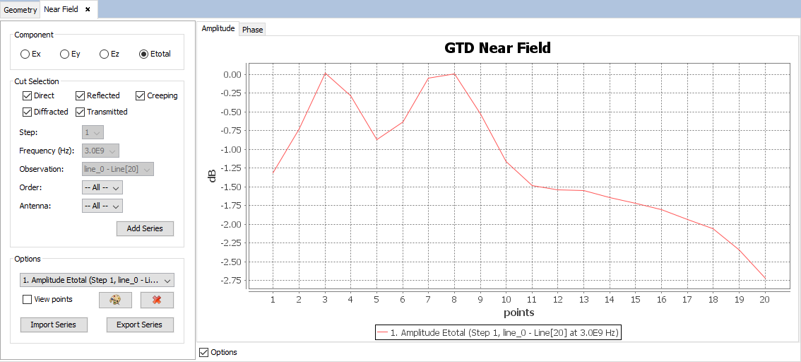
Step 14: To visualize the angular cuts, click on Show Results → Near Field → View Cuts.