To perform interactive compensator design functions, consider a system with the open-loop transfer function:
You are required to design a lag compensator for this system such that a phase margin of 45o is maintained. Assume that Kc = 1.
The angle θGH is computed from the equation:
θGH = -180o + 45o + 5o = -130o
To interactively design a lag compensator
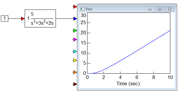
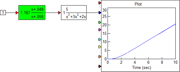
1. Create and simulate the following system:
2. Set the polynomial coefficients for the transferFunction block to the following values:
Numerator: 1
Denominator: 1 3 2 0
Note: Always leave spaces between coefficient values.
3. Select the transferFunction block.
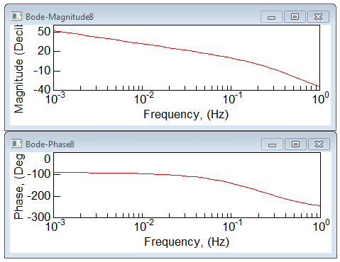
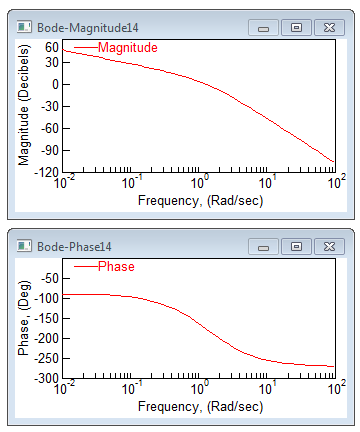
4. Choose Analyze > Frequency Response to display the Bode magnitude and phase plots.
5. Move and resize them for better viewing.
As can be seen from the Bode phase plot, the frequency corresponding to a phase of -130o is approximately 0.48 rad. Therefore, ω1 = 0.48. The corresponding magnitude of the open-loop transfer function, from the Bode magnitude plot, is 0.853.
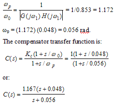
The lag zero frequency is ω0 = 0.1 ω1 = 0.048. The lag pole frequency is given by:

6. Select the transferFunction block.
7. Choose Analyze > Compensator Design.
8. In the Compensator Design dialog with the plant poles and zeros displayed, do the following:
•In the Compensator Zeros box, enter (-0.048,0) and click Add.
A 0 is displayed in the Compensator Zeros list. The entry corresponds to a 0 in the complex plane, with a real part of -0.048 and an imaginary part of 0.
•In the Compensator Poles box, enter (-0.056,0) and click Add.
This pole is displayed in the Compensator Poles list.
•In the Gain box, enter 1.167.
•Click Replot.
The Bode magnitude and phase plots of the Compensator-Plant system, C(s) GH(s) are displayed. The Bode plots indicate that the phase margin is approximately 48o.
9. Click OK in the Compensator Design dialog.
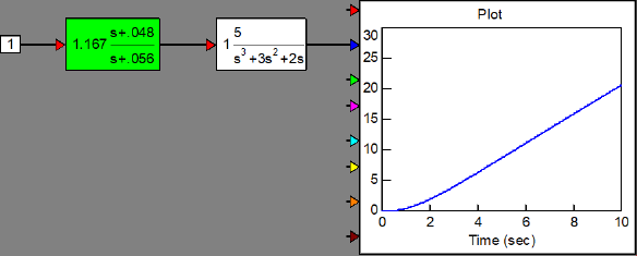
10. Place the new Compensator block before the plant transfer function GH(s), and connect it as shown below. The Compensator-Plant system is now ready for use or further analysis.