Introduction
Introduction
![]()
Library
HydraulicsByFluidon/UsersGuide
Description
The package HydraulicsByFluidon is a modelica library for the one-dimensional simulation of fluid-power systems. The models are based on the lumped parameter approach. The library consists of various hydraulic components and predefined hydraulic fluids. In order to enable the user to create custom components, the library specific component interfaces are provided as well.
Minimal working example
Each model created by using the HydraulicsByFluidon package requires the Liquid and Environment blocks to be added:
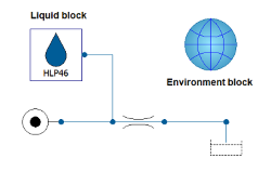
The environment block provides the simulation with information about the environmental conditions, e.g. the ambient pressure or the value of the gravitational constant. The liquid block determines the hydraulic fluid that is used, which is why every hydraulic component in a model has to be connected to it. In order to save the user the trouble of connecting the liquid block to each component manually, the option forwardFluidProperties is included in certain components. If this option is used, the user has to connect the liquid block to each hydraulic circuit only once since the fluid information is forwarded between the components.
Fundamentals of the lumped parameter approach
In hydraulic engineering, the lumped parameter approach assumes that the state of a cross-section within a hydraulic system is fully described by the (mass) flow rate and the pressure. Due to numerical limitations, the application of the lumped parameter approach is usually restricted to systems with low to moderate dynamic effects. In the lumped parameter approach, there are three fundamental types of hydraulic elements:
- Resistor
- Capacitor
- Inductor

This equation states that the mass flow rate is assumed to be proportional to the n-th power of the pressure drop across the component. The exponent can vary between 1 and 0.5, depending on the flow regime.
By contrast, the capacitor corresponds to an ideal hydraulic spring without any losses or inertia. Mathematically, its behaviour is described by the following differential equation:
According to this model, the temporal change in pressure is proportional to the difference in incoming and outgoing mass flows, multiplied with the bulk modulus and divided by the density and volume of the fluid in the respective component.
The inductor is an ideal inertia without any losses or stiffness. It is mathematically described by the following equation:

This equation is the hydraulic formulation of Newton's second law of motion. It states that the temporal change in mass flow rate is equal to the pressure difference across the component, multiplied by the cross-sectional flow area and divided by the length of the component.
Solution procedure
These fundamental elements can be used alone or in combination to model actual hydraulic components. If components modeled through these elements are connected to a circuit model, they form a system of coupled ordinary differential equations which has to be solved numerically. The solving algorithm works in a staggered way: based on the initial pressure distribution, the resistors and inductors calculate flow rates. These flow rates are then used as boundary conditions for the capacitors, which calculate the new pressure distribution in return. After this step, the whole procedure is repeated. Due to the algorithm structure outlined above, reasonable initial pressures have to be assigned to components that are based on capacitor elements, e.g. simple volumes.
Instructions regarding the use of individual components can be found in the respective component's documentation.
Component library
The User's Guides for the Component library can be accessed here.